When you press and hold buttons A or C, they allow you to further change the attributes of the two respective video oscillators. That is by pressing and holding A, you affect the first oscillator, while pressing and holding C affects the second oscillator. The manual for the Hypno calls this Shape Pages, but I will call this Mod Mode, as the settings that are accessed through this method essentially modulate the oscillator. For those of you who are new to the concept of modulation, we can simplify the concept for the Hypno, and state that modulation makes the images move.
When pressing and holding A or C, the functions mirror each other. For instance, when you hold down button A, slider A controls the scrolling of the shape. However, when you hold down button C, you would now using slider B to do the same affect. Thus, when describing various functions, I will try to describe slider and dial positions in relationship to the button being held, while also putting the exact slider or dial in parenthesis in order to be clear.
So, as already stated, the slider on the same side of the button controls the scrolling of the shape (slider A for button A, slider B for button C). The dial that is closest to the button (dial A for button A, dial D for button C) changes the speed at which the shape rotates. The top dial on the same side as the button (dial B for button A, dial C for button C) controls the amount of modulation for polarization or for Y (vertical) scrolling. In the later case, the twelve o’clock position on the dial indicates no scrolling, while moving the dial to the left causes the shape to scroll down, while moving the dial to the right causes the shape to scroll up.
The the top dial on the opposite side as the button (dial C for button A, dial B for button C) controls the amount of fractal modulation. The dial on the opposite side of the button (dial D for button A, dial A for button C) controls the amount of fractal drift, or if fractal modulation is off, the amount of mirroring or repetition. The slider on the opposite side of the button (slider B for button A, slider A for button C), controls the amount of modulation sent the selected oscillator to the other oscillator (A to B or B to A). The top dial (E) sets the color saturation for the selected oscillator (ranging from white fully saturated). Finally, the lower dial (F) sets the hue offset from the root hue setting from performance mode.
As we get further into modulation, it is very possible to make settings in modulation mode that you find difficult to impossible to undo or un tangle. Rebooting the Hypno by turning it off and turning it back on again, can allow you to reset it, but often dealing with the lack of predictability is part of the process. That being said, if you want to feel more in control of the output, change the settings in modulation mode slowly and change only one setting at a time, while noticing the visual change that occurs with that setting change.
A silent video demonstration of most of the options in modulation mode on the Hypno.
Here’s a Sleepy Circuits quick guide describing how to control color using a combination of Performance and Modulation Modes . . .
video by Sleepy Circuits
Likewise, here’s a Sleepy Circuits quick guide showing how fractal modulation is achieved in Modulation Mode . . .
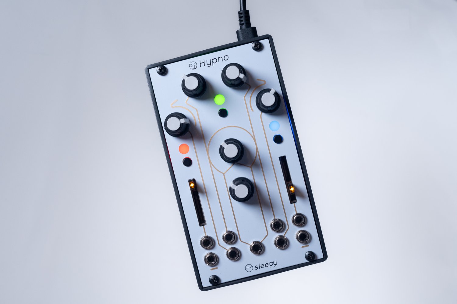
As previously stated, the face of the Hypno features two sliders, three buttons, and six dials. For convenience, through this manual, I will refer to the two sliders as A & B (left to right) and the three buttons as A, B, & C (left to right). For the dials I will refer to the four at the top as A, B, C, & D (left to right) and the two in the center as E & F (middle to bottom). The Hypno has several modes of operation that are accessed by holding down (or not holding down) buttons. I will refer to the mode where no buttons are being held down as performance mode.
image from Sleepy Circuits.
To get started with the Hypno, let’s not use any input, and just use it to generate video using its two video oscillators. The module is symmetrical, so the controls on the left (slider A, button A, and dials A & B) generally control the first oscillator, while the controls on the right (slider B, button C, and dials C & D) control the second oscillator. The controls in the middle (button B and dials E & F) generally control the module as a whole.
Buttons A & C set the shape for the two oscillators. Pressing the buttons cycles through the shapes, sine, tan, poly, circle / oval, fractal noise, and video input. These shapes are coded with the color of corresponding LED (red, green, yellow, blue, pink, and teal). The last setting, teal / video input, is only accessible when a USB video input is plugged in. We’ll deal with the video input shape in a later tutorial. While the manufacturer refers to the first two shapes as sine and tan, they both are essentially lines. The polygon shape is a septagon by default.
Red
Sine
Green
Tan
Yellow
Polygon
Blue
Circle / Oval
Pink
Fractal Noise
Teal
Video Input
A silent video demonstration of the five basic shapes in Hypno.
Sliders A & B set what the manufacturer calls frequency, but perhaps it is better understood as a zoom function. The zoom feature can be very useful when you are first getting used to the Hypno. Zooming in completely, that is pulling the slider all the way to the bottom can make a video layer disappear, so you can better see the effect of each control. Dials A & D rotate the selected shapes, and dials B & C control the polarization of the shapes. When polarization is low, the shapes appear normal. As polarization increases, the shapes start to bend until they completely wrap around, forming concentric circles. However, it should be noted that for the polygon, circle / oval, and video input shapes, dials B & C function as Y (vertical) offsets.
A silent video demonstration of the zoom, rotate and polarization / y offset controls on the five basic shapes.
The remaining two dials (E & F) control both oscillators. The former controls the gain of each shape, with the center position resulting in a black out of both layers. The latter dial controls affects the colors of the two layers, shifting the relationship between the hues of the two layers. At this point you should understand the basic shapes and controls in performance mode for the Hypno. Notice however, with the controls we have introduced thus far, there is no movement on its own. That is the shapes only change when a control (button, slider, or dial) is changed.
Here is the Sleepy Circuits quick guide for performance mode (they call it shape pages) . . .
The Sleepy Circuits Hypno is a video synthesizer that can generate video using two video oscillators that generate a variety of shapes shapes. Each video oscillator can be manipulated using a series of buttons, sliders, and dials. The Hypno can also accept video input via USB for each of the two video oscillators, allowing it to manipulate video (live or pre-recorded) in real time. Sleepy Circuits has a lot of great info about how to use the Hypno spread between the manufacturer’s website and their YouTube channel. However, in my opinion, they lack a single resource that functions like a full manual taking you through how to use the Hypno from beginning to end. I hope to do this in a few blog entries.
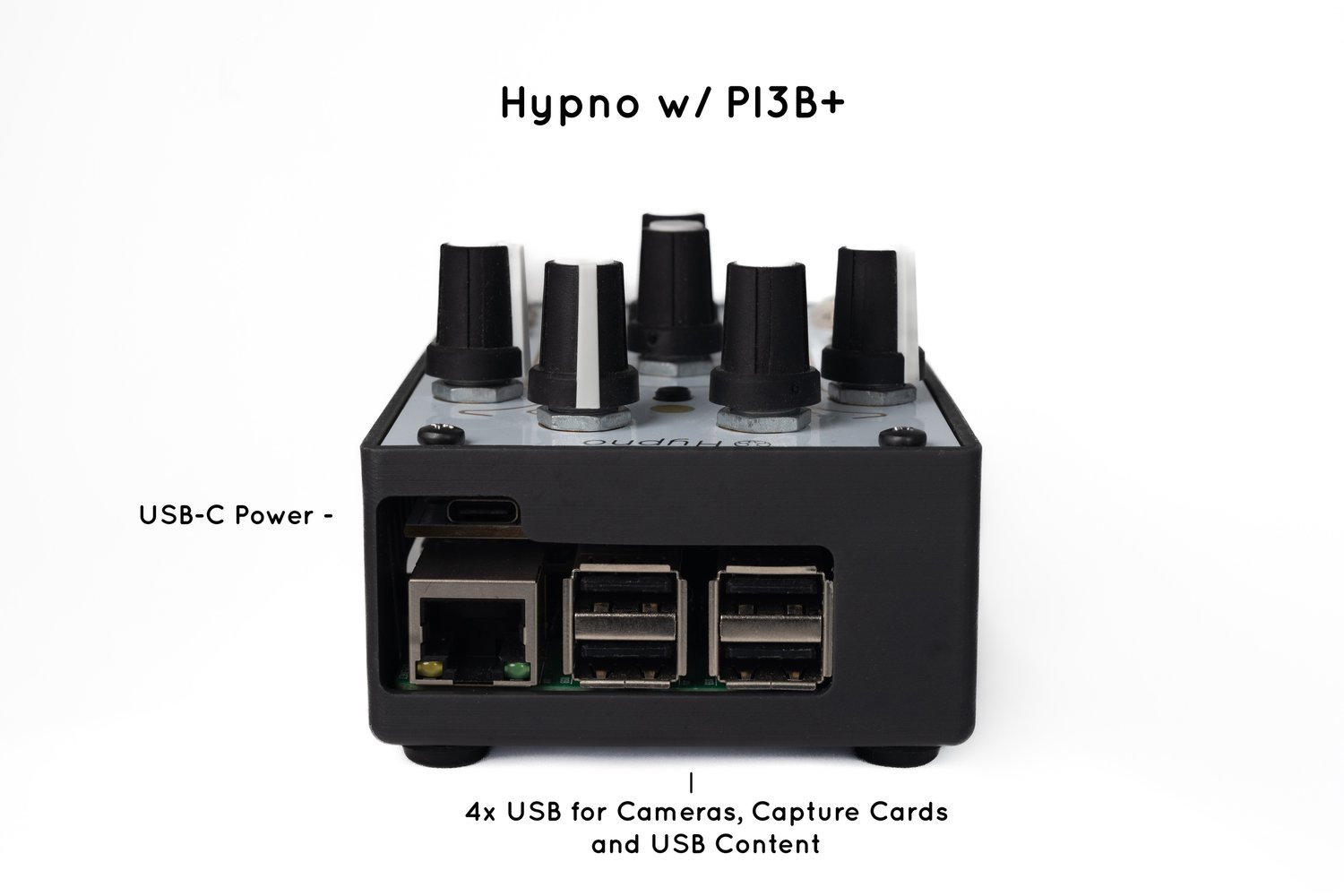
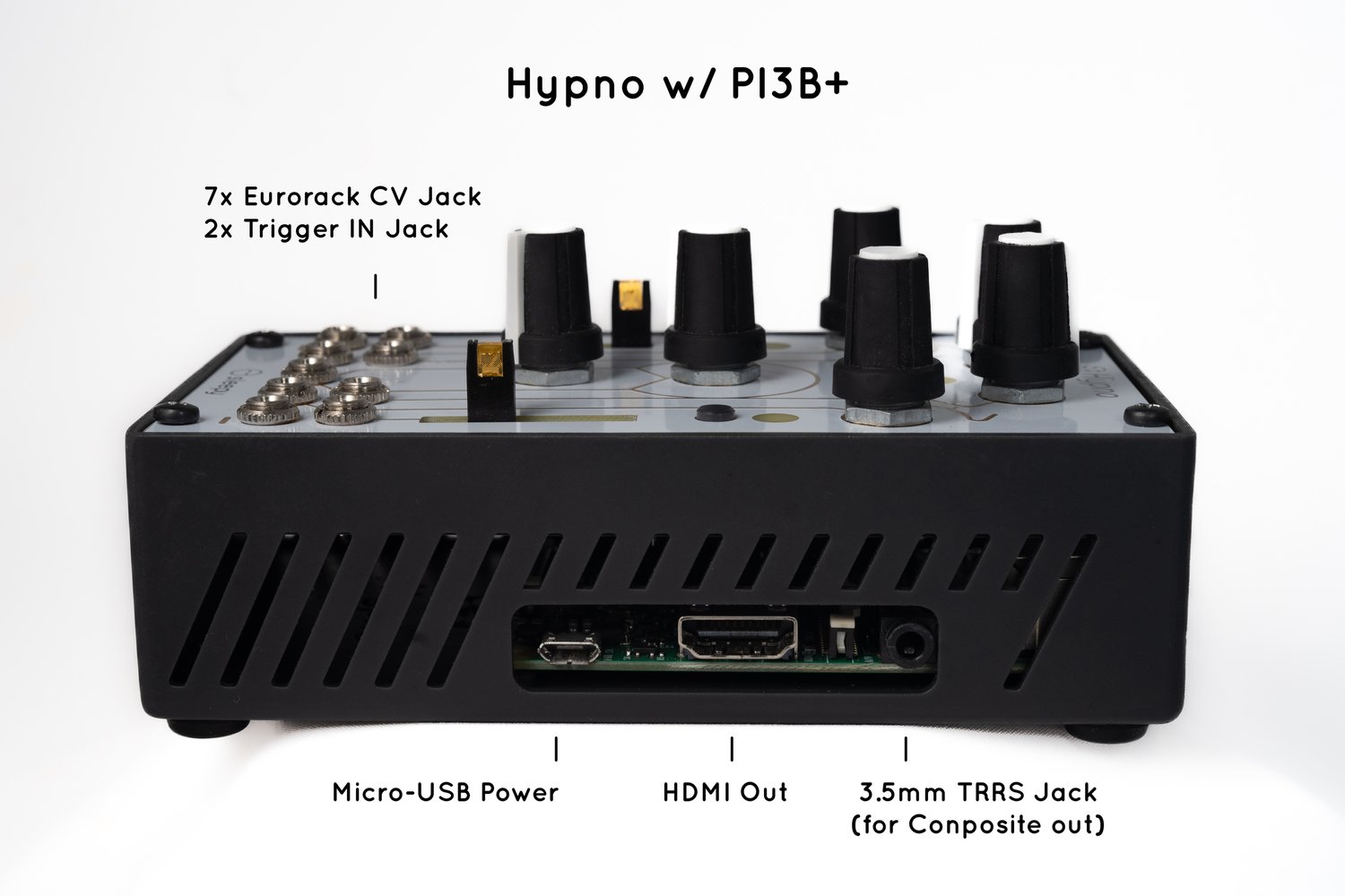
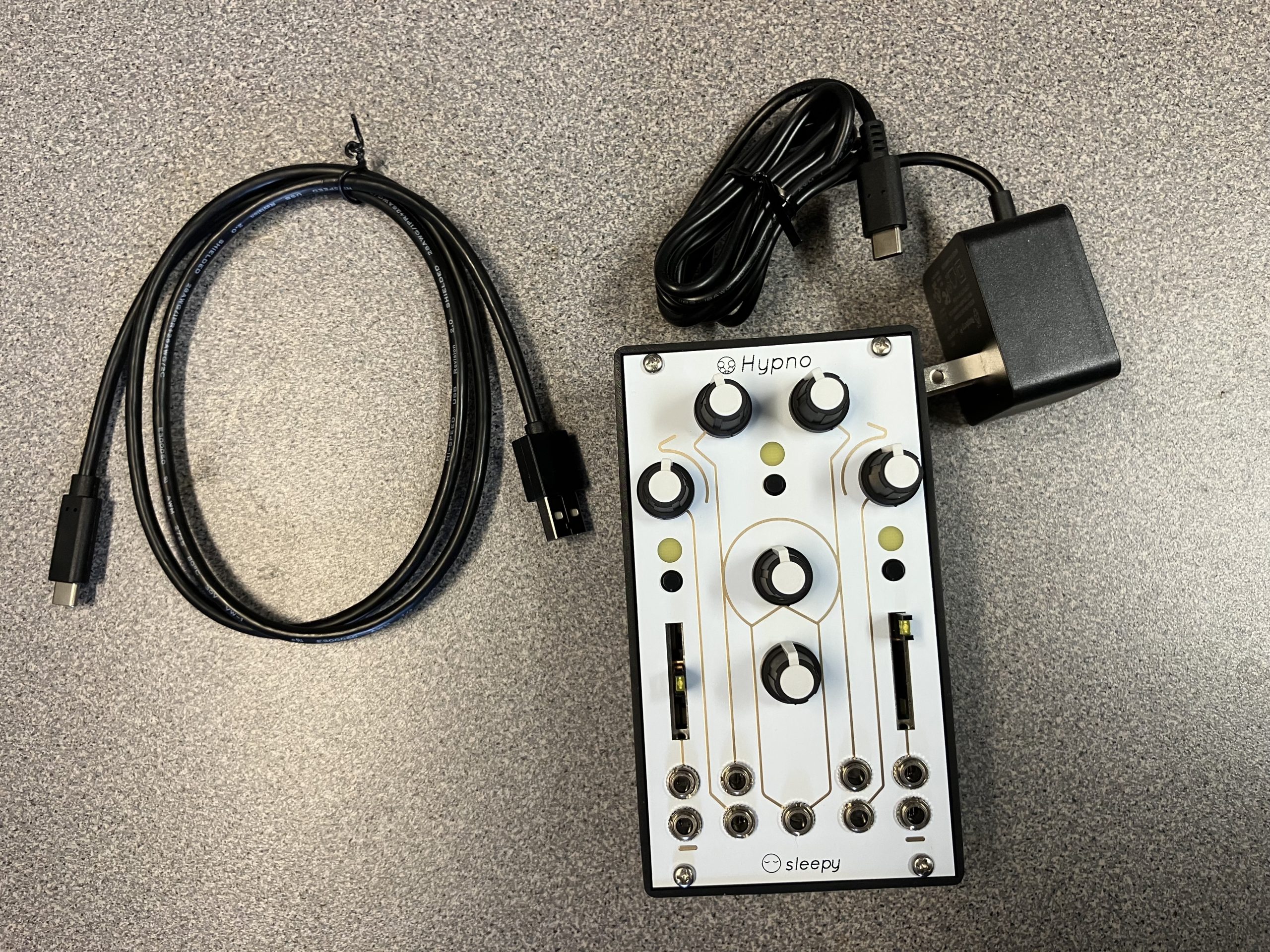
Let’s start off by looking at inputs and outputs. The back face of the Hypno features four USB inputs that can be used for connecting cameras, capture cards, USB drives, and MIDI instruments. The right hand side of the module features an HDMI out, a composite out, and a micro USB port which is used to power the unit. The Hypno is a bit picky in terms of the order you plug things in. You should always plug in the HDMI out before plugging in the power. When you plug in the power, you will notice that the Hypno goes through a boot up process. Note that there is no power switch, so turning the unit on and off is done through plugging it in and unplugging it. If you are going to use any USB input, you would plug that in third, after plugging in the power.
image from Sleepy Circuits.
image from Sleepy Circuits.
The face of the Hypno features two sliders, three buttons, and six dials. Since each of these fulfills several functions, none of them are labelled. The face also has nine 3.5mm TS sockets for use with Eurorack and Eurorack compatible gear. These nine ports can be used to control / automate the two sliders, two of the three buttons, and five of the six dials. We’ll spend more time dealing with this in a future post. However, if you plan on using these Eurorack connections, you will want to connect them after connecting power.
image from Sleepy Circuits.
At this point, you should be able to correctly connect the Hypno to inputs, outputs, and power in the correct order.
Darth Presley & Deejayeetee will be performing together live on February 21st at 7:30PM at the ShowUp Gallery in Boston for the opening of the Bait/Switch exhibit. They will be performing . . .
“Windghost,” Wyste,” and “Catoblepas” are tracks from the forthcoming Darth Presley album Monstrum Pacificum Bellicosum (projected December 2026). “Muddle” was Deejayeetee’s project for the yellow Bait/Switch project.
I’m pleased to announce that myself and Professor Katherine Elia-Shannon from Stonehill College’s Communication Department have been awarded a Digital Innovation Grant from the Digital Innovation Lab at the MacPháidín library. The grant will continue my investigation of video synthesis that I started using the Critter and Guitari EYESY from my previous Digital Innovation Grant. This time around I will be using the Sleepy Circuits Hypno.
The Hypno generates video in realtime, and features four USB inputs with an HDMI output. The core of the video generation is two video oscillators that generate what Sleepy Circuits call shapes. These two shapes are superimposed over each other. Various parameters, such as shape, frequency, rotation, and polarization can be controlled for each video oscillator. Likewise, there are global parameters that can be manipulated such as gain, hue, saturation, feedback. These parameters can also be controlled via MIDI over USB or via control voltages from a Eurorack compatible modular synthesizer. In addition to the internal shapes offered by the video oscillators, the Hypno can accept video input via USB as a shape for each of the two video oscillators, allowing the user to manipulate live or pre-recorded video in real time.
The first step will be to create a series of blog entries that explain the various features of the Hypno. This post will be aided by the vast resources on the YouTube channel for Sleepy Circuits. After that, I plan on making music videos for the four pieces on my most recent album, Point Nemo. I will also be teaching the features of the Hypno to Professor Katherine Elia-Shannon and her students for them to use in an assignment.
The first batch of equipment, the Hypno and a power cable, arrived this past week. In July the second half of the grant funding will payout, so at that stage I will be purchasing accessories to use with the Hypno. Stay posted for updates!
I gave a presentation at Synthfest on November 9th, 2024 in Burlington, Massachusetts. This workshop is related to my ongoing research in using Pure Data as a tool for computer-assisted composition, sound processing, and sound synthesis. Specifically, the presentation is on how to use Pure Data to create polymetric beats. A hackable template is available below for download. You can hear such beats in my most recent album, Rotate (Bandcamp, Spotify, Apple, Amazon).
Pure Data is often used as a tool for sound synthesis or signal processing. A quick history lesson reminds us however that it is also a robust tool for algorithmic, or computer-assisted composition. Pure Data is an open source visual programming environment for sound and multimedia. It is strongly based upon the programming environment Max. When Max first added the ability to process and generate audio and video, it was referred to as Max/MSP/Jitter to highlight these new abilities. However, going back to the very beginnings of Max, originally developed at IRCAM in 1985 by Miller Puckette (who also developed Pure Data), it was centered on interactive, algorithmic and computer-assisted composition.
Defining the Problem
In order to create polymetric beats in Pure Data, it is useful to think of two steps in the process. The first is how do we represent musical patterns in a way that is easy to codify for computers. The second is how do we read that pattern in such a way that we can fire off a MIDI note at the correct time to realize that pattern.
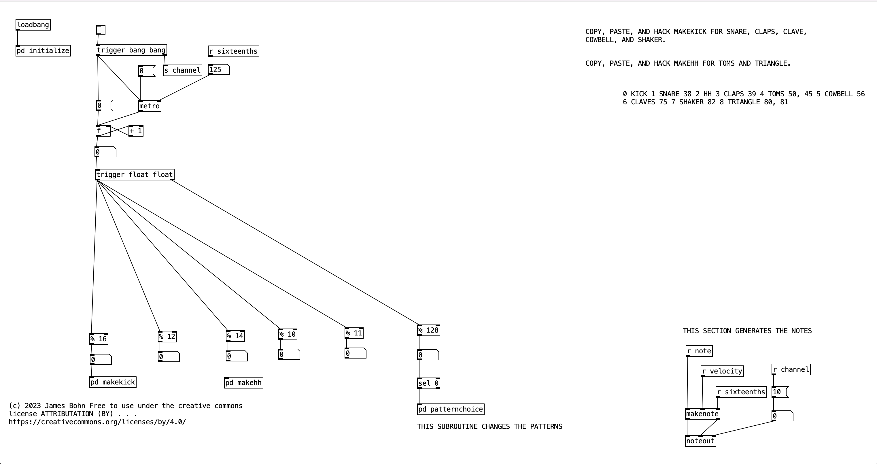
Attached to this blog post is a program shell that we will use to understand a basic process where patterns are defined and initialized, a time structure, a structure for evaluating whether a note should happen, an algorithm for firing off a note, and a structure for changing musical patterns. The way this program shell is designed, it currently only generates kick drum parts in common time. However, once we learn how this algorithm works, we can hack it to create far more complicated beats.
Defining a Pattern
Generating rhythmic content using an algorithm is a very useful exercise, as we do not have to worry about pitch material. On the most basic level, we could think of a measure of as being a list of sixteenth notes (or whatever the fastest pulse of the desired rhythm is), and we can express the rhythm by using zeros where notes do not happen, and ones where notes are played. Thus, if we want to define a four on the floor kick drum part in common time, we could express it as . . .
1 0 0 0 1 0 0 0 1 0 0 0 1 0 0 0
When we define tables in Pure Data, the first number indicates where in the table we’re putting the values. Typically, we would want to start at the beginning of the table, which would be position 0. Thus, from now on in, I will start every rhythm description with a 0, resulting in . . .
0 1 0 0 0 1 0 0 0 1 0 0 0 1 0 0 0
This is pretty basic. If we wanted to go a bit more advanced, we could imagine two different options, a normal kick drum, which we’ll represent with the number 1, and an accented kick drum, which we’ll represent with the number 2. If we want to accent beat one of the measure, we now get the table description . . .
0 2 0 0 0 1 0 0 0 1 0 0 0 1 0 0 0
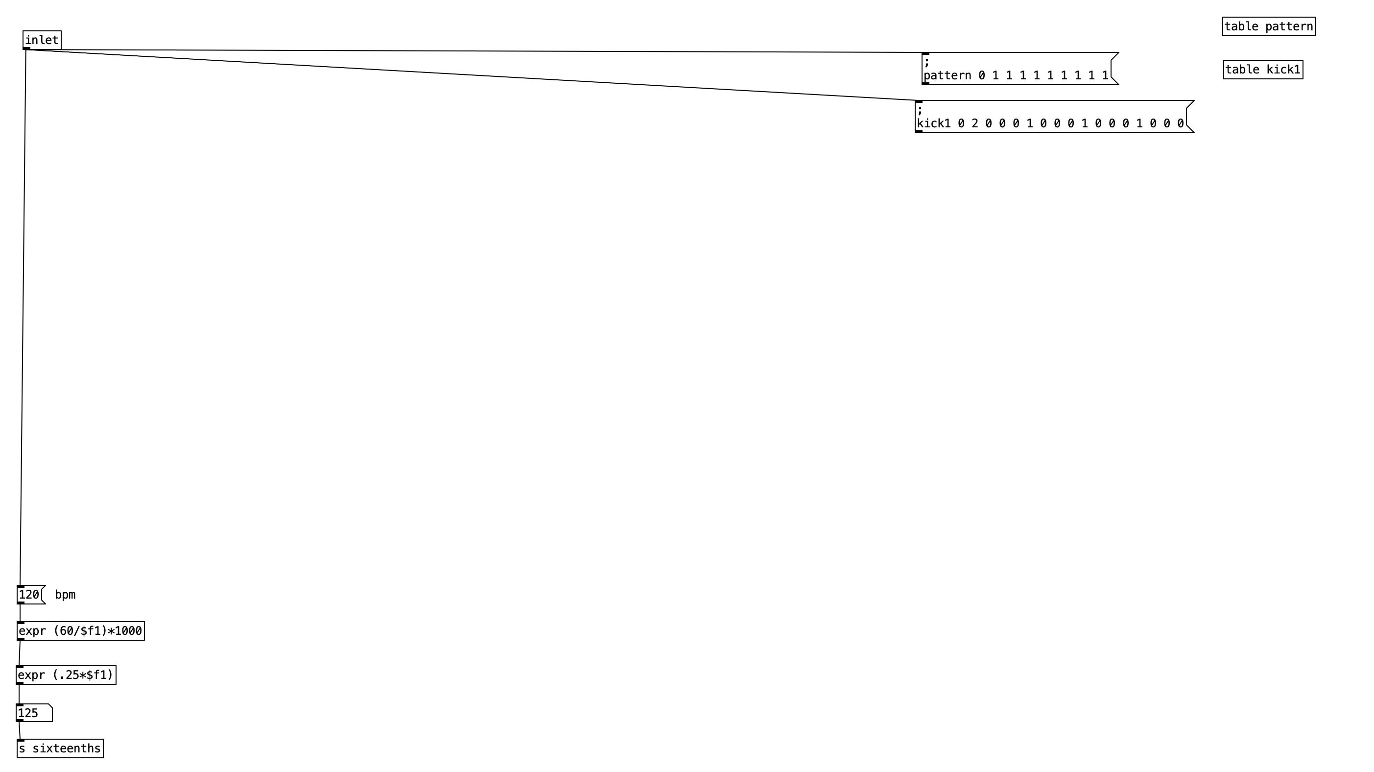
Notice, it would be pretty easy at this point to use the number zero for when notes do not occur, but use the MIDI velocity number(1-127) to indicate when a note should occur. Doing this, you can get very finely tuned dynamic drum parts. However, such subtlety is not for me, I’m more of a boom / bap / boom-boom / bap guy myself, so I will be sticking with accented and unaccented notes. Let’s look at this table definition as it occurs in the program shell. To get there, double click on the object labeled pd initialize, which is below loadbang . . .
For those who are relatively new to Pure Data, loadbang designates algorithms that execute when you open the program. Likewise, any object in Pure Data that starts with the letters pd are subroutines. Double clicking them allows you to view and edit the algorithm contained inside the subroutine. Subroutines are a great way to declutter your screen, and to create algorithms that you may want to copy and paste into other programs you create. Note that the subroutine pd initializealso sets the tempo, translates that into milliseconds, and then into sixteenth notes (still expressed in milliseconds). Finally, we also see that pd initialize contains a definition for a table called phrase, but we’ll get to that later.
Changing Patterns
Before we get to how to use this kick drum pattern, I want to introduce one more level of complexity. In the long term it would be useful to define several different kick drum patterns so we can change patterns every eight measures or so to have a dynamic drum part. As we start to add more layers to the drum part (snare, high hat, toms, etc.) it would also be nice if some of those layers occasionally did not play at all, so the combination of layers also change as we move from phrase to phrase.
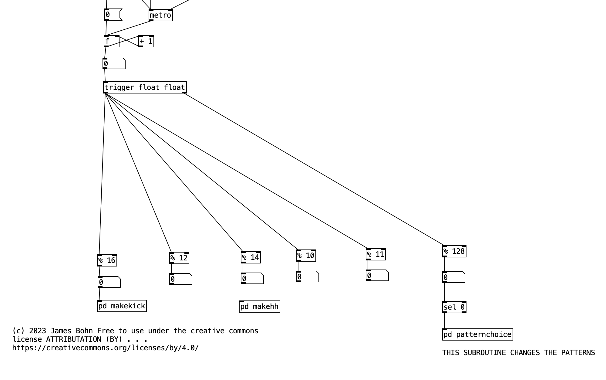
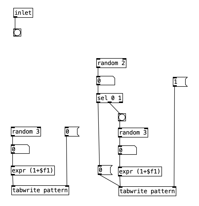
For the purposes of this algorithm, I’m going to allow for each layer of the drum part to select between three patterns (1, 2, & 3). Furthermore, I’ll also include a fourth possibility of 0, which would correspond to no pattern playing. In order to see how this is implemented in our algorithm, let’s look at the counter mechanism beneath the main metronome object. Beneath this metronome we see a trigger object, and beneath that, we see an object that states % 128. This is modular mathematics, which limits the value to a number between 0 and 127 (inclusive). We then feed the outcome of this to an object that states sel 0. When this object receives a 0 in its leftmost inlet, it will send a bang to its leftmost outlet. We then send this bang to trigger the subroutine pd patternchoice. Musically, what this means, is that the subroutine pd patternchoice executes at the beginning of every eight measure phrase. Since we are thinking in terms of sixteenth notes (8 x 16 = 128), a 0 would indicate the beginning of a phrase.
If we look inside pd patternchoice, we see two structures that are currently not connected to the inlet. In time we will copy and paste these structures, changing some of the numeric values, and connect them to the inlet. We will make these changes as we add more layers and patterns to our drum beat. However, for the time being since we only have one kick drum pattern, neither structure is connected to the inlet.
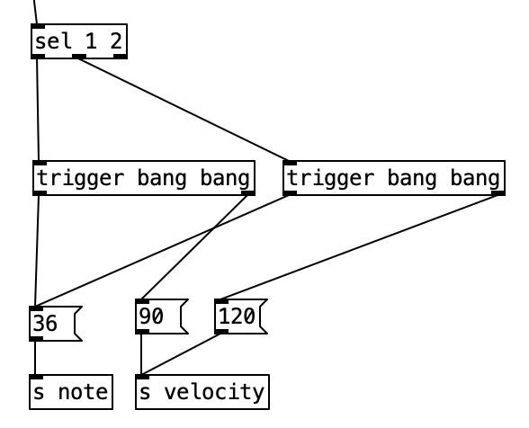
We will treat the algorithm on the left as being connected to the kick drum, while the algorithm on the right will eventually be used for the snare drum. Notice there is a difference between the two structures. The one on the left is simpler, and if we follow what it does, we figure out that that algorithm will write a 1, 2, or 3, but not a 0 to the table pattern in position 0. The structure on the right however, will write a 0 to the table patttern at position 1 half of the time. To put this into musical terms, the difference between the two means that kick drum will always be playing a pattern, while the snare drum will only play a pattern 50% of the time.
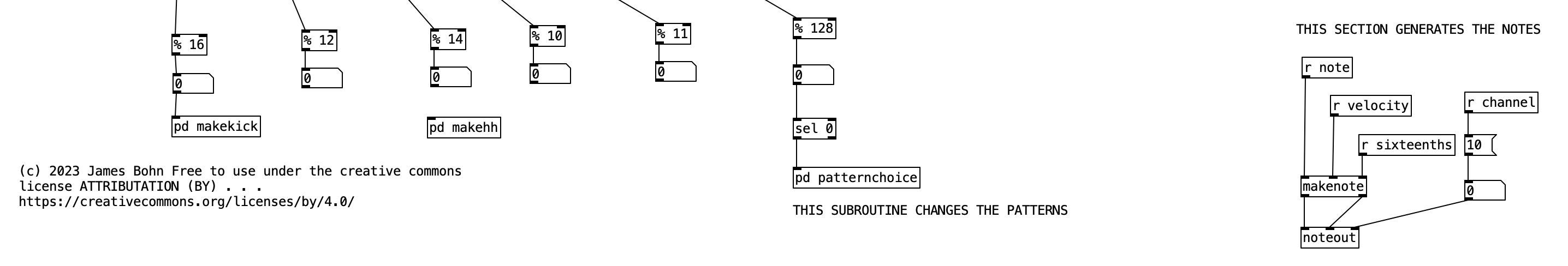
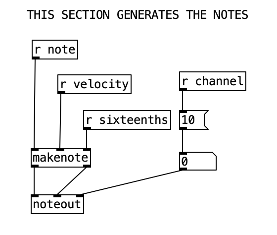
Firing Off a Note
Now lets see how pattern and kick1 are used to either fire off notes or not. We see at the bottom of the screen a makenote object connected to a noteout object that performs the final task of sending a midi note out. However pd makekick is the subroutine that determines whether or not a kick drum should occur at a given point. Above pd makekick we see the object % 16 which comes from the counter. This object mods the current counter to a number between 0 and 15 inclusive. These values correspond to the number of sixteenth notes in a measure of common time. Thus, when we return to the number 0 after the number 15 occurs it corresponds to returning to the beginning of the measure.
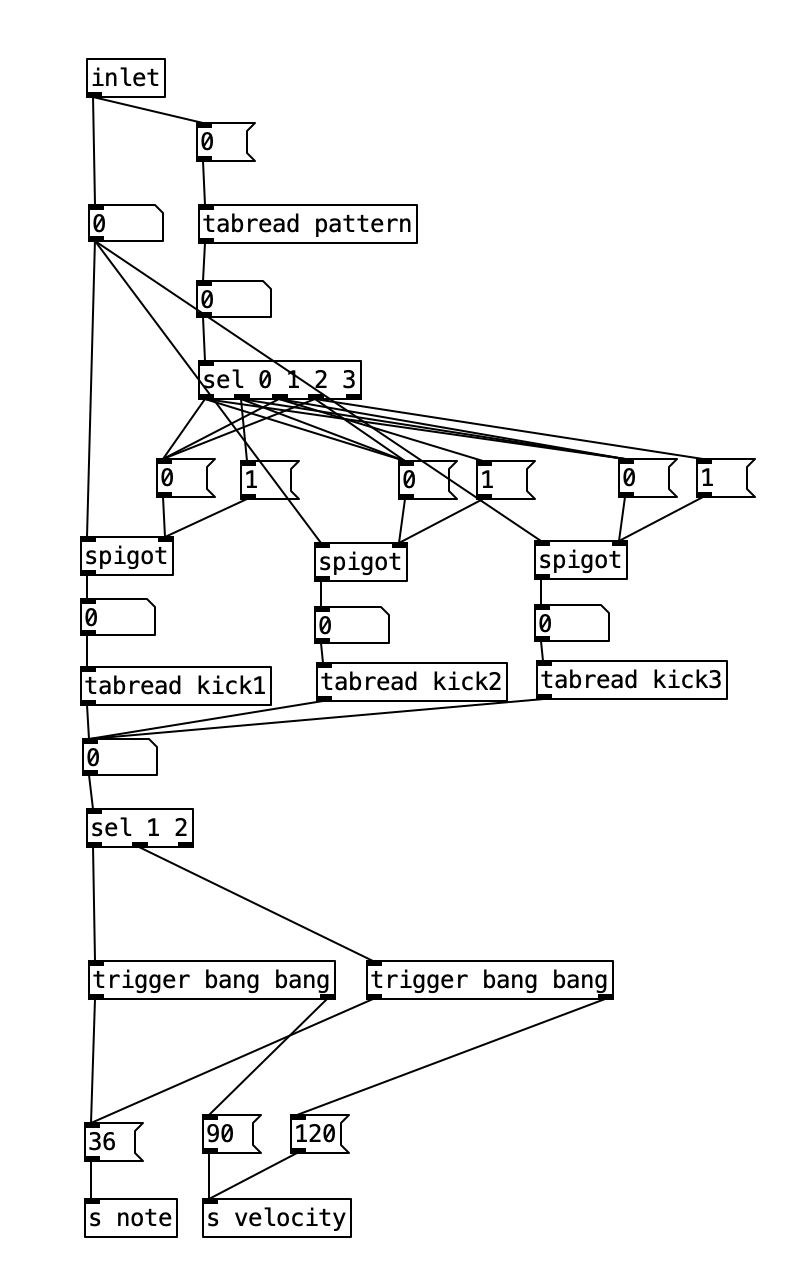
When we look at the structure pd makekick a lot of the heavy lifting of the subroutine is handled by the object spigot. Spigot receives numeric values through its leftmost inlet. However, it only passes those values through to its outlet if the numeric value being fed to its right most inlet is not zero. Thus, we can think of spigot as a valve that shuts off the flow of numbers when the rightmost inlet is zero. We can use this to selectively shut down the rest of the algorithm, which will effectively stop it from making notes.
The first step is to determine whether a pattern should be playing or not. Likewise, at the same time we can determine which patterns should be playing if one occurs. To do this, we’ll read the value of pattern at array position 0 (which we’ll use to store the current kick drum pattern). We can then route the output of that to a number of different outcomes using a sel statement. Each outcome of the sel statement sends either a 0 or a 1 to the rightmost inlet of three spigots. These spigots correspond to the three possible kick drum patterns. Thus, when the pattern is 0, a 0 is sent to all three spigots, effectively shutting off the rest of the subroutine. When the pattern is 1, we send a 1 to the spigot for pattern one (turning it on), and a zero to the other two, making sure any previously used pattern is turned off, and so fourth.
Once we pass through one of the spigots, we encounter the part of the subroutine that determines whether a note should be fired at any given time. Underneath each spigot is a tabread object that reads the current position of a given pattern (kick1, kick2, or kick3, respectively). This will return the result of a 0, 1, or 2, corresponding to no note, normal note, and accented note. Since we don’t have to do anything when no note is played, we can simply ignore that result. All we have to do is correctly route the results for 1 and 2. Since all three patterns will be outputing 0, 1, and 2, we will treat those three results the same, we can route the output of each tabread statement to the same number box, and then route the results using sel 1 2. Both results will sending the number 36 to s note (36 is the MIDI note number corresponding to a kick drum), and will send a velocity of either 90 or 120 to s velocity.
Understanding Execution Order
In order to understand the mechanics of this, we have to understand a little about execution order for Pure Data. When an outlet branches off in several directions, Pure Data first executes the connection that was created first, regardless of where it is placed on the screen (in Max, it executes from right to left). When an algorithm branches off in this way, it travels all the way down until it hits the end, and then Pure Data goes back and executes the other branch of the algorithm. When an object has multiple outlets, it typically executes the rightmost outlet first (following it all the way down the algorithm) before it most to the next outlet.
Alternately, when an object has several inlets, the object typically does not spring into action until the leftmost inlet is triggered. We can think of new values that are connected to inlets that are note the leftmost inlet as queueing until the leftmost inlet is triggered. This order of execution in Pure Data allows non-crossed connections to fire in the correct order. To illustrate, imagine an object with two outlets and an object below with two inlets (similar to the makenote / noteout algorithm below). Furthermore, let’s imagine that the right outlet is connected to the right inlet of the object below, and the left outlet is connected to the left inlet of the object below. First, the value from the right outlet will queue at the right inlet of the object below, then the left outlet will send its value to the left inlet, triggering the object below.
However, whenever we start to make complicated algorithms, it can be confusing to see in what order the algorithm will flow. When we want to force a specific order to achieve a specific outcome, or simply to make order clear, we can use a trigger object. A trigger takes a single inlet, and uses it to trigger several outlets (including the option of passing the inlet to one or more outlets) in a specific order. That order is (you guessed it, right to left). We will use this to control the order of sending the velocity and sending the note number.
The makenote object has three inlets that correspond to midi note number, velocity, and duration expressed in milliseconds. Since midi note number is the leftmost inlet, we have to send that value last. This means we have to send the velocity before we send the note number. Here we do not have to worry about duration, since duration is often irrelevant when triggering drum samples. Thus, we can set a duration of a sixteenth note during the initialization process.
Hacking the Shell
With the knowledge we have gained thus far, we are now equipped to start hacking the program shell. A good place to start would be to double click [pd initialize], copy both the object [table kick1] and the corresponding message that populates that table. You can then paste these objects, move them so they don’t overlap, change both to say kick2 instead of kick1, and change the numbers in the in the kick2 message to be a different pattern. Again, your pattern should only use the numbers 0, 1, and 2. Likewise, the table should be 17 numbers long with the first number being 0, in order to denote that we’ll load the array starting at the beginning. You can then connect the kick2 message to the [inlet] object.
Now do the same process again creating a table and message for kick3, making sure to connect the kick3 message to inlet. Now, we can finally make use of the subroutine [pd patternchoice] in the main algorithm. Double click on [pd patternchoice], and connect the outlet of the bang to both the [random 3] object and the message that contains the number 0. Now, when we run the the algorithm, we should hear the kick drum pattern randomly change once every eight measures.
Now we can get into the good stuff. Let’s add a snare drum part. First, we should decide what meter we want to use for the snare drum. For the purposes of this demonstration, let’s put the snare drum in three. We’ll start by copying the object [pd makekick] and pasting it. More the copied object under the [% 12] object, and connect the outlet of [% 12] to the inlet of the copied object. Let’s also rename the copied object to [pd makesnare].
We have to change some details of [pd makesnare] to get it to make a snare part. Double click the object and change the message box near the top from 0 to 1. Change the array names in the three [tabread] objects to be snare1, snare2, and snare3. Finally, right above the object [s note], change the number in the message box from 36 to 38 (the MIDI note number for snare drum).
Now, double click the object [initialize], and copy the three kick drum tables, as well as the three messages that define those tables. Paste those items, and move them so they don’t overlap with other items. change the array names to snare1, snare2, and snare3 in both the table objects and the messages that define the arrays. Now, let’s change the patterns. Since these are patterns that are in three, they will feature 12 sixteenth notes. Thus, each message will have to include 13 numbers, the first being the number 0 to indicate that the pattern is loaded at the beginning of the array. Again, use 0 to indicate no note, 1 to indicate a note, and 2 to represent an accented note. Make sure you connect each of the three messages to the inlet.
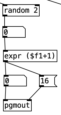
Now we need to allow the snare patterns to change, so let’s double click the subroutine [pd patternchoice]. In this subroutine we need to connect the outlet of the bang to both the [random 2] object and the message that contains the number 1. The[random 2] here yields a 50% chance that the snare appear in a given phrase. The [random 3] below that will select one of the three snare patterns when it is determined that the snare should appear in a phrase.
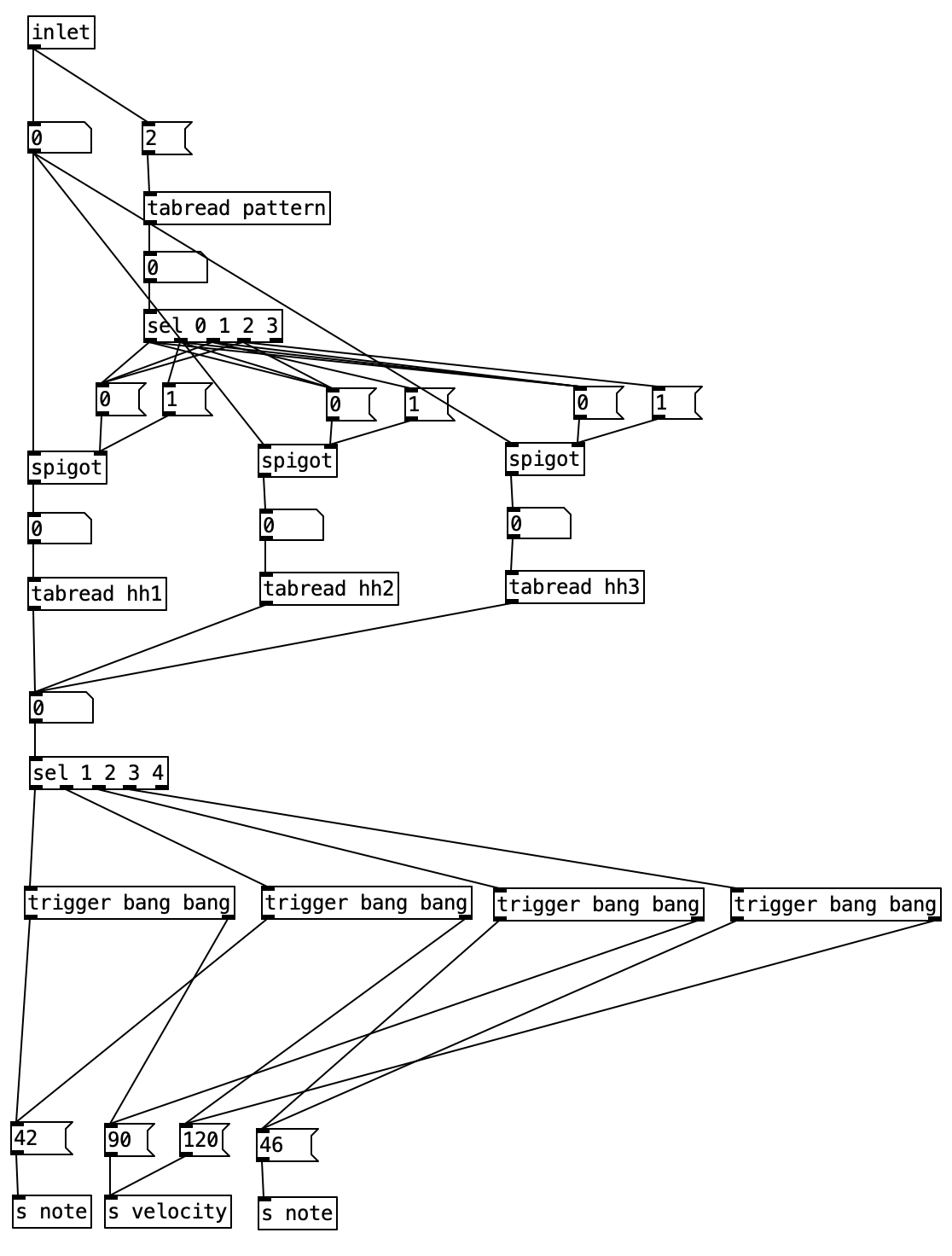
If we wanted to make a percussion part that used two different MIDI notes, we should look at the subroutine, [pd makehh]. Two notes are required for a high hat part to allow for closed and open high hats. If we look inside pd makehh, we see that the patterns allow for five possibilities, 0, 1, 2, 3, & 4. When we look at the sel statement near the bottom of the screen, the number 0 does not appear in it. Again, this is because 0 means do not play a note, so we can simply ignore that result. The way this is setup, 1 and 2 are closed high hats with the latter being accented, while 3 and 4 are open high hats with 4 being accented.
If we wanted to fully implement this subroutine, we’d have to attach it to one of the meter generators, % 16, % 12, % 14, % 10, or % 11. Then we would have to create three patterns (hh1, hh2, hh3) in [pd initialize], remembering to make the table, and use a message to populate it. You would populate the patterns using only the numbers 0, 1, 2, 3, and 4. Then you’d have to copy the block of code inside of pd patternchoice that we used to choose the pattern for the snare drum, paste it, change the index in the message object to 2, and connect the random object and the index message to the inlet.
We could also adapt [pd makehh] for creating a subroutine that will generate a toms or conga part consisting of a high tom / conga and a low tom / conga. You would have to remember to use a new / different index number to store the pattern, and change the MIDI note numbers to those corresponding to either the a high tom or conga and a low tom or conga. Ultimately we can continue in this vein, creating increasingly complicated drum beats, using [pd makekick] as a means creating layers of single note percussion parts, and [pd makehh] as a model for creating percussion layers using two different notes. As the number of meters used increases, you’ll find the resulting beats get increasingly funky, and take longer times to evolve in compelling ways, enabling you to inject rhythmic interest into your music.
As I mentioned in my previous experiment, it has been a busy and difficult semester for me for family reasons. Accordingly, I am two and a half months behind schedule delivering my 12th and final experiment for this grant cycle. Additionally, I feel like my work for the past few months on this process has been a bit underwhelming, but unfortunately this work what my current bandwidth allows for. I hope to make up for it in the next year or so.
Anyway, the experiment for this month is similar to the one done for experiment 11. However, in this experiment I am generate vector images that reference maps of Boston’s subway system (the MBTA). Due to the complexity of the MBTA system I’ve created four different algorithms, reducing the visual data at any time to one quadrant of the map, thus, the individual programs are called: MBTA NW, MBTA NE, MBTA SE, & MBTA SW.
Since all four algorithms are basically the same, I’ll use MBTA – NE as an example. For each example Knob 5 was used for the background color. There were far more attributes I wanted to control than knobs I had at my disposal, so I decided to link them together. Thus, for MBTA – NE knob 1 controls red line attributes, knob 2 controls the blue and orange line attributes, knob 3 controls the green line attributes, and knob 4 controls the silver line attributes. Each of the four programs assigns the knobs to different combinations of colored lines based upon the complexity of the MBTA map in that quadrant.
The attributes that knobs 1-4 control include: line width, scale (amount of wiggle), color, and number of superimposed lines. The line width ranges from one to ten pixels, and is inversely proportional to the number of superimposed lines which ranges from on to eight. Thus, the more lines there are, the thinner they are. The scale, or amount of wiggle is proportional to the line width, that is the thicker the lines, the more they can wiggle. Finally, color is defined using RGB numbers. In each case, only one value (the red, the green, or the blue) changes with the knob values. The amount of change is a twenty point range centered around the optimal value. We can see this implemented below in the initialization portion of the program.
	RElinewidth = int (1+(etc.knob1)*10)
	BOlinewidth = int (1+(etc.knob2)*10)
	GRlinewidth = int (1+(etc.knob3)*10)
	SIlinewidth = int (1+(etc.knob4)*10)
	etc.color_picker_bg(etc.knob5)
	REscale=(55-(50*(etc.knob1)))
	BOscale=(55-(50*(etc.knob2)))
	GRscale=(55-(50*(etc.knob3)))
	SIscale=(55-(50*(etc.knob4)))
	thered=int (89+(10*(etc.knob1)))
	redcolor=pygame.Color(thered,0,0)
	theorange=int (40+(20*(etc.knob2)))
	orangecolor=pygame.Color(99,theorange,0)
	theblue=int (80+(20*(etc.knob2)))
	bluecolor=pygame.Color(0,0,theblue)
	thegreen=int (79+(20*(etc.knob3)))
	greencolor=pygame.Color(0,thegreen,0)
	thesilver=int (46+(20*(etc.knob4)))
	silvercolor=pygame.Color(50,53,thesilver)
	j=int (9-(1+(7*etc.knob1)))
The value j stands for the number of superimposed lines. This then transitions into the first of four loops, one for each of the groups of lines. Below we see the code for red line portion of program. The other three loops are fairly much the same, but are much longer due to the complexity of the MBTA map. An X and a Y coordinate are set inside this loop for every point that will be used. REscale is multiplied by a value from etc.audio_inwhich is divided by 33000 in order to change that audio level into a decimal ranging from 0 to 1 (more or less). This scales the value of REscale down to a smaller value, which is added to the numeric value. It is worth noting that because audio values can be negative, the numeric value is at the center of potential outcomes. Scaling the index number of etc.audio_in by (i*11), (i*11)+1, (i*11)+2, & (i*11)+3 lends a suitable variety of wiggles for each instance of a line.
	j=int (9-(1+(7*etc.knob1)))
	for i in range(j):
		AX=int (320+(REscale*(etc.audio_in[(i*11)]/33000)))
		AY=int (160+(REscale*(etc.audio_in[(i*11)+1]/33000)))
		BX=int (860+(REscale*(etc.audio_in[(i*11)+2]/33000)))
		BY=int (720+(REscale*(etc.audio_in[(i*11)+3]/33000)))
		pygame.draw.line(screen, redcolor, (AX,AY), (BX, BY), RElinewidth)
I arbitrarily limited each program to 26 points (one for each letter of the alphabet). This really causes the vector graphic to be an abstraction of the MBTA map. The silver line in particular gets quite complicated, so I’m never really able to fully represent it. That being said, I think that anyone familiar with Boston’s subway system would recognize it if the similarity was pointed out to them. I also imagine any daily commuter on the MBTA would probably recognize the patterns in fairly short order. However, in watching my own video, which uses music generated by a PureData algorithm that will be used to write a track for my next album, I noticed that the green line in the MBTA – NE and MBTA – SW needs some correction.
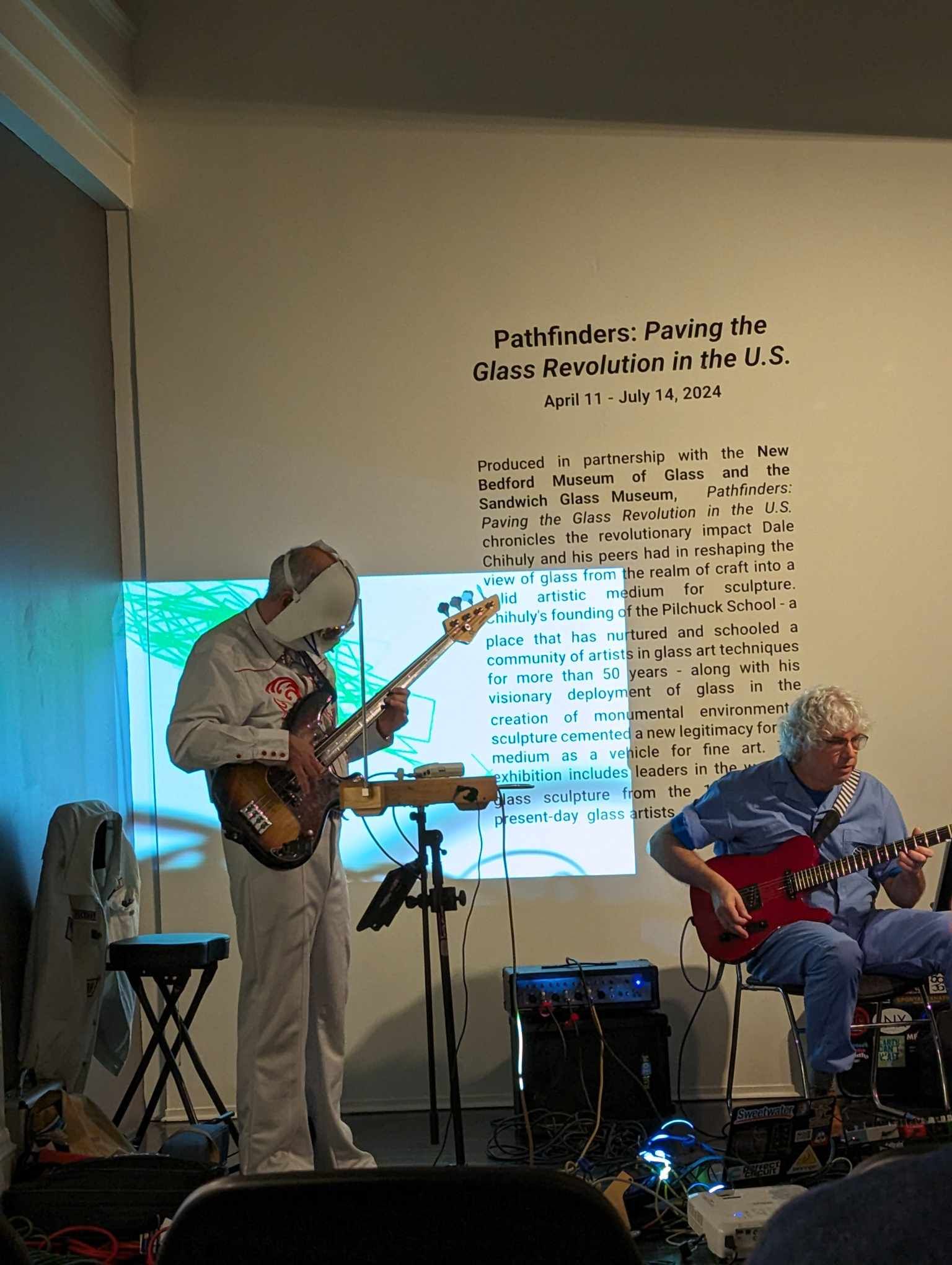
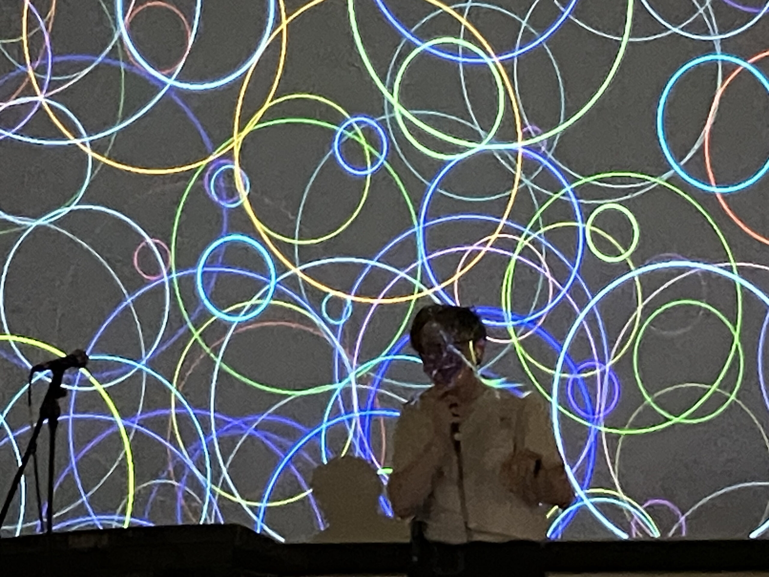
The EYESY has been fully incorporated into my live performance routine as Darth Presley. You can see below a performance at the FriYay series at the New Bedford Art Museum. You’ll note that the projection is the Random Lines algorithm that I wrote. Likewise graduating senior Edison Roberts used the EYESY for his capstone performance as the band Geepers! You’ll see a photo of him below with a projection using the Random Concentric Circles algorithm that I wrote. I definitely have more ideas of how to use the EYESY in live performance. In fact, others have started to use ChatGPT to create EYESY algorithms.
Ultimately my work on this grant project has been fruitful. To date the algorithms I’ve written for the Organelle and EYESY have been circulated pretty well on Patchstorage.com (clearly the Organelle is the more popular format of the two) . . .
Bio: I have had some horribly disturbing waking dreams of being a monstrous apparition, part-man, but mostly machine; soulless and demonic, terrorizing man and beast alike with sounds unlike any other, sounds that alternately inspire and chill, lifting spirits only to dash them again on some distant rocky shore comprised of dissonance and psychotic visions. I am haunted by sizable blackouts, what some refer to as lost time, and frequently awaken in unknown locations, smelling of Malört and regret with nothing to explain my activities save for a plectrum and a few patch chords.
The H.E.A.P. (The Housatonic Electronic Algorithmic Philharmonic): Dr. Todd Gernes: electric guitar Darth Presley: fretless bass, theremin Volca Sample 2, Volca Keys, Volca FM 2, EYESY (video synthesizer) driven by algorithms written in Pure Data.
TriStar, 737, A300, DC-8, 727, 707, DC-10, DC-9, & 747 are from the album Rotate (Bandcamp, Spotify, Apple Music, Amazon Music). Roc, Delver, Ankheg, Windghost, Bulette, Wyste, Aboleth, Rampager, Catoblepas, Megalodon, Moonbeast, & Hydra are from the forthcoming album Monstrum Pacificum Bellicosum (projected completion 2026). The untitled ambient piece will hopefully be released on an album planned for 2025.
Special thanks to: Scott Bishop, Dr. Todd Gernes, Dr. Uma Hiremath, Dr. Greg Maneiro, Garrett McComas, and the Digital Innovation Lab at Stonehill College.
February was a very busy month for me for family reasons, and it’ll likely be that way for a few months. Accordingly, I’m a bit late on my February experiment, and will likely be equally late with my final experiment as well. I have also stuck with programming for the EYESY, as I have kind of been on a roll in terms of coming up with ideas for it.
This month I created twelve programs for the EYESY, each of which displays a different constellation from the zodiac. I’ve named the series Constellations and have uploaded them to patchstorage. Each one works in exactly the same manner, so we’ll only look at the simplest one, Aries. The more complicated programs simply have more points and lines in them with different coordinates and configurations, but are otherwise are identical.
Honestly, one of the most surprising challenges of this experiment way trying to figure out if there’s any consensus for a given constellation. Many of the constellations are fairly standardized, however others are fairly contested in terms of which stars are a part of the constellation. When there were variants to choose from I looked for consensus, but at times also took aesthetics into account. In particular I valued a balance between something that would look enticing and a reasonable number of points.
I printed images of each of the constellations, and traced them onto graph paper using a light box. I then wrote out the coordinates for each point, and then scaled them to fit in a 1280×720 resolution screen, offsetting the coordinates such that the image would be centered. These coordinates then formed the basis of the program.
import os
import pygame
import time
import random
import math

def setup(screen, etc):
    pass

def draw(screen, etc):
	linewidth = int (1+(etc.knob4)*10)
 	etc.color_picker_bg(etc.knob5)
	offset=(280*etc.knob1)-140
	scale=5+(140*(etc.knob3))
	r = int (abs (100 * (etc.audio_in[0]/33000)))
	g = int (abs (100 * (etc.audio_in[1]/33000)))
	b = int (abs (100 * (etc.audio_in[2]/33000)))
	if r>50:
		rscale=-5
	else:
		rscale=5
	if g>50:
		gscale=-5
	else:
		gscale=5
	if b>50:
		bscale=-5
	else:
		bscale=5
	j=int (1+(8*etc.knob2))
	for i in range(j):
		AX=int (offset+45+(scale*(etc.audio_in[(i*8)]/33000)))
		AY=int (offset+45+(scale*(etc.audio_in[(i*8)+1]/33000)))
		BX=int (offset+885+(scale*(etc.audio_in[(i*8)+2]/33000)))
		BY=int (offset+325+(scale*(etc.audio_in[(i*8)+3]/33000)))
		CX=int (offset+1165+(scale*(etc.audio_in[(i*8)+4]/33000)))
		CY=int (offset+535+(scale*(etc.audio_in[(i*8)+5]/33000)))
		DX=int (offset+1235+(scale*(etc.audio_in[(i*8)+6]/33000)))
		DY=int (offset+675+(scale*(etc.audio_in[(i*8)+7]/33000)))
		r = r+rscale
		g = g+gscale
		b = b+bscale
		thecolor=pygame.Color(r,g,b)
		pygame.draw.line(screen, thecolor, (AX,AY), (BX, BY), linewidth)
		pygame.draw.line(screen, thecolor, (BX,BY), (CX, CY), linewidth)
		pygame.draw.line(screen, thecolor, (CX,CY), (DX, DY), linewidth)
In these programs knob 1 is used to offset the image. Since only one offset is used, rotating the knob moves the image on a diagonal moving from upper left to lower right. The second knob is used to control the number of superimposed versions of the given constellation. The scale of how much the image can vary is controlled by knob 3. Knob 4 controls the line width, and the final knob controls the background color.
The new element in terms of programing is a for statement. Namely, I use for i in range (j) to create several superimposed versions of the same constellation. As previously stated, the amount of these is controlled by knob 2, using the code j=int (1+(8*etc.knob2)). This allows for anywhere from 1 to 8 superimposed images.
Inside this loop, each point is offset and scaled in relationship to audio data. We can see for any given point the value is added to the offset. Then the scale value is multiplied by data from etc.audio_in. Using different values within this array allows for each point in the constellation to react differently. Using the variable i within the array also allows for differences between the points in each of the superimposed versions. The variable scale is always set to be at least 5, allowing for some amount of wiggle given all circumstances.
Originally I had used data from etc.audio_in inside the loop to set the color of the lines. This resulted in drastically different colors for each of the superimposed constellations in a given frame. I decided to tone this down a bit, by using etc.audio_in data before the loop started allowing each version of the constellation within a given frame to be largely the same color. That being said, to create some visual interest, I use rscale, gscale, and bscale to move the color in a direction for each superimposed version. Since the maximum amount of superimposed images is 8, I used the value 5 to increment the red, green, and blue values of the color. When the original red, green, or blue value was less than 50 I used 5, which moves the value up in value. When the original red, green, or blue value was more than 50 I used -5, which moves the value down in value. The program chooses between 5 and -5 using if :else statements.
The music used in the example videos are algorithms that will be used to generate accompaniment for a third of my next major studio album. These algorithms grew directly out of my work on these experiments. I did add one little bit of code the these puredata algorithms however. Since I have 6 musical examples, but 12 EYESY patches, I added a bit of code that randomly chooses between 1 of 2 EYESY patches and sends out a program (patch) change to the EYESY on MIDI channel 16 at the beginning of each phrase.
While I may not use these algorithms for the videos for the next studio album, I will likely use them in live performances. I plan on doing a related set of EYESY programs for my final experiment next month.
I kind of hit a wall of the Organelle. I feel like in order to advance my skills I have a bit of a hurdle between where my programming skills are at, and where they would need to be to do something more advanced that the recent experiments I have completed. Accordingly for this month I decided to shift my focus to the EYESY. Last month I made significant progress in understanding Python programming for the EYESY, and that allowed me to come up with five ideas for algorithms in short order. The music for all five mini-experiments comes from PureData algorithms I will be using for my next major album. All five of these algorithms are somewhat derived from my work on my last album.
The two realizations that allowed me to make significant progress on EYESY programming is that Python is super picky about spaces, tabs, and indentations, and that while the EYESY usually gives little to no feedback when a program has an error in it, you can use an online Python compiler to help figure out where your error is (I had mentioned the latter in last month’s experiment). Individuals who have a decent amount of programming experience may scoff at the simplicity of the programs that follow, but for me it is a decent starting place, and it is also satisfying to me to see how such simple algorithms can generate such gratifying results.
Random Lines is a patch I wrote that draws 96 lines. In order to do this in an automated fashion, I have to use a loop, in this case I use for i in range(96):. The five lines that follow are all executed in this loop. Before the loop commences, we choose the color using knob 4 and the background color using knob 5. I use knob 3 to set the line width, but I scale it by multiplying the knob’s value, which will be between 0 and 1, by 10, and adding 1, as line widths cannot have a value of 0. I also have to cast the value as an integer. I set an x offset value using knob 1. Multiplying by 640 and then subtracting 320 will yield a result between -320 and 320. Likewise, a y offset value is set using knob 2, and the scaling results in a value between -180 and 180.
import os
import pygame
import time
import random
import math

def setup(screen, etc):
    pass

def draw(screen, etc):
	color = etc.color_picker(etc.knob4)
	linewidth = int (1+ (etc.knob3)*10)
 	etc.color_picker_bg(etc.knob5)
	xoffset=(640*etc.knob1)-320
	yoffset=(360*etc.knob2)-180
   	for i in range(96):
		x1 = int (640 + (xoffset+(etc.audio_in[i])/50))
		y1 = int (360 + (yoffset+(etc.audio_in[(i+1)])/90))
		x2 = int (640 + (xoffset+(etc.audio_in[(i+2)])/50))
		y2 = int (360 + (yoffset+(etc.audio_in[(i+3)])/90))
		pygame.draw.line(screen, color, (x1,y1), (x2, y2), linewidth)
Within the loop, I set two coordinates. The EYESY keeps track of the last hundred samples using etc.audio_in[]. Since these values use sixteen bit sound, and sound has peaks (represented by positive numbers) and valleys (represented by negative numbers), these values range between -32,768 and 32,787. I scale these values by dividing by 50 for x coordinates. This will scale the values to somewhere between -655 and 655. For y coordinates I divide by 90, which yields values between -364 and 364.
In both cases, I add these values to the corresponding offset value, and add the value that would normally, without the offsets, place the point in the middle of the screen, namely 640 (X) and 360 (Y). A negative value for the xoffset or the scaled etc.audio_in value would move that point to the left, while a positive value would move it to the right. Likewise, a negative value for the yoffset or the scale etc.audio_in value would move the point up, while a positive value would move it down.
Since subsequent index numbers are used for each coordinate (that is i, i+1, i+2, and i+3), this results in a bunch of interconnected lines. For instance when i=0, the end point of the drawn line (X2, Y2) would become the starting point when i=2. Thus, the lines are not fully random, as they are all interconnected, yielding a tangled mass of lines.
Random Concentric Circles uses a similar methodology. Again, knob five is use to control the background color, while knobs 1 and 2 are again scaled to provide an X and Y offset. The line width is shifted to knob 4. For this algorithm the loop happens 94 times. The X and Y value for the center of the circles is determined the same way as was done in Random Lines. However, we now need a radius and we need a color for each circle.
import os
import pygame
import time
import random
import math

def setup(screen, etc):
    pass

def draw(screen, etc):
	linewidth = int (1+(etc.knob4)*9)
 	etc.color_picker_bg(etc.knob5)
	xoffset=(640*etc.knob1)-320
	yoffset=(360*etc.knob2)-180
	for i in range(94):
		x = int (640 + xoffset+(etc.audio_in[i])/50)
		y = int (360 + yoffset+(etc.audio_in[(i+1)])/90)
		radius = int (11+(abs (etc.knob3 * (etc.audio_in[(i+2)])/90)))
		r = int (abs (100 * (etc.audio_in[(i+3)]/33000)))
		g = int (abs (100 * (etc.audio_in[(i+4)]/33000)))
		b = int (abs (100 * (etc.audio_in[(i+5)]/33000)))
		thecolor=pygame.Color(r,g,b)
		pygame.draw.circle(screen, thecolor, (x,y), radius, linewidth)
We have knob 3 available to help control the radius of the circle. Here I multiply knob 3 by a scaled version of etc.audio_in[(i+2)]. I scale it by dividing by 90 so that the largest possible circle will mostly fit on the screen if it is centered in the screen. Notice that when we multiply knob 3 by etc.audio_in, there’s a 50% chance that the result will be a negative number. Negative values for radii don’t make any sense, so I take the absolute value of this outcome using abs. I also add this value to 11, as a radius of 0 makes no sense, and a radius of less than 10, as having a line width that is larger than the radius will cause an error.
For this algorithm I take a set forward by giving each circle its own color. In order to do this I have to set the value for red, green, and blue separately, and then combine them together using pygame.Color(). For each of the three values (red, green, and blue) I divide a value of etc. audio_in by 33000, which will yield a value between 0 and 1 (more or less), and then multiply this by 100. I could have done the same thing by simply dividing etc.audio_in by 330, however, at the time this process made the most sense to me. Again, this process could result in a negative number and / or a fractional value, so I cast the result as an integer after getting its absolute value.
Colored Rectangles has a different structure than the previous two examples. Rather than have all the objects cluster around a center point I wanted to create an algorithm that spaces all of the objects out evenly throughout the screen in a grid like pattern. I do this using an eight by eight grid of 64 rectangles. I accomplish the spacing using modulus mathematics as well as integer division. The X value is obtained by multiplying 160 times i%8. In a similar vein, the Y values is set to 90 times i//8. Integer division in Python is accomplished through the use of two slashes. Using this operator will return the integer value of a division problem, omitting the fractional portion. Both the X and the Y values have an additional offset value. The X is offset by (i//8)*(80*etc.knob1), so this offset increases as knob 1 is turned up, with a maximum offset of 80 pixels per row. The value i//8 essentially multiplies that offset by the row number. That is the rows shift further towards the right.
import os
import pygame
import time
import random
import math

def setup(screen, etc):
    pass

def draw(screen, etc):
 	etc.color_picker_bg(etc.knob5)
   	for i in range(64):
		x=(i%8)*160+(i//8)*(80*etc.knob1)
		y=(i//8)*90+(i%8)*(45*etc.knob2)
		thewidth=int (abs (160 * (etc.knob3) * (etc.audio_in[(i)]/33000)))
		theheight=int (abs (90 * (etc.knob4) * (etc.audio_in[(i+1)]/33000)))
		therectangle=pygame.Rect(x,y,thewidth,theheight)
		r = int (abs (100 * (etc.audio_in[(i+2)]/33000)))
		g = int (abs (100 * (etc.audio_in[(i+3)]/33000)))
		b = int (abs (100 * (etc.audio_in[(i+4)]/33000)))
		thecolor=pygame.Color(r,g,b)
		pygame.draw.rect(screen, thecolor, therectangle, 0)
Likewise, the Y offset is determined by (i%8)*(45*etc.knob2). As the value of knob 2 increases, the offset moves towards a maximum value of 45. However, as the columns shift to the right, those offsets compound due to the fact that they are multiplied by (i%8).
A rectangle can be defined in pygame by passing an X value, a Y value, width, and height to pygame.Rect. Thus, the next step is to set the width and height of the rectangle. In both cases, I set the maximum value to 160 (for width) and 90 (for height). However, I scaled them both by multiplying by a knob value (knob 3 for width and knob 4 for height). These values are also scaled by an audio value divided by 33,000. Since negative values are possible from audio values, and negative widths and heights don’t make much sense, I took the absolute value of each. If I were to rewrite this algorithm (perhaps I will), I would set a minimum value for width and height such that widths and heights of 0 were not possible.
I set the color of each rectangle using the same method as I did in Random Concentric Circles. In order to draw the rectangle you pass the screen, the color, the rectangle (as defined by pygame.Rect), as well as the line width to pygame.draw.rect. Using a line width of 0 means that the rectangle will be filled in with color.
Random Rectangles is a combination of Colored Rectangles and Random Lines. Rather than use pygame’s Rect object to draw rectangles on the screen, I use individual lines to draw the rectangles (technically speaking they are quadrilaterals). Knob 4 is used here to set the foreground color, knob 5 is used here to set the background color, knob 3 is used to set the linewidth.
import os
import pygame
import time
import random
import math

def setup(screen, etc):
    pass

def draw(screen, etc):
	color = etc.color_picker(etc.knob4)
 	etc.color_picker_bg(etc.knob5)
	linewidth = int (1+ (etc.knob3)*10)
   	for i in range(64):
		x=(i%8)*160+(i//8)*(80*etc.knob1)+(40*(etc.audio_in[(i)]/33000))
		y=(i//8)*90+(i%8)*(45*etc.knob2)+(20*(etc.audio_in[(i+1)]/33000))
		x1=x+160+(40*(etc.audio_in[(i+2)]/33000))
		y1=y+(20*(etc.audio_in[(i+3)]/33000))
		x2=x1+(40*(etc.audio_in[(i+4)]/33000))
		y2=y1+90+(20*(etc.audio_in[(i+5)]/33000))
		x3=x+(40*(etc.audio_in[(i+6)]/33000))
		y3=y+90+(20*(etc.audio_in[(i+7)]/33000))
		pygame.draw.line(screen, color, (x,y), (x1, y1), linewidth)
		pygame.draw.line(screen, color, (x1,y1), (x2, y2), linewidth)
		pygame.draw.line(screen, color, (x2,y2), (x3, y3), linewidth)
		pygame.draw.line(screen, color, (x3,y3), (x, y), linewidth)
Within the loop, I use a similar method of setting the initial X and Y coordinates. That being said, I separate out the use of knobs and the use of audio input. In the case of the X coordinated, I use (i//8)*(80*etc.knob1) to control the amount of x offset for each row, with a maximum offset of 80. The audio input then offsets this value further using (40*etc.audio_in[(i+2)]/33000). This moves the x value by a value of plus or minus 40 (remember that audio values can be negative. Likewise, knob 2 offsets the Y value for every row by a maximum of 45, and the audio input further offsets this value by plus or minus 20.
Since it takes four points to define a quadrilateral, we need three more points, which we will call (x1, y1), (x2, y2), and (x3, y3). These are all interrelated. The value of X is used to define X1 and X3, while X2 is based off of X1. Likewise, the value of Y helps define Y1 and Y3, with Y2 being based off of Y1. In the case X1 and X2 (which is based on X1) we add 160 to X, giving a default width, but these values are again scaled by etc.audio_in. Similarly, we add 90 to Y1 and Y3 to determine a default height of the quadrilaterals, but again, all points are further offset by etc.audio_in, resulting in quadrilaterals, rather than rectangles with parallel sides. If I were to revise this algorithm I would likely make each quadrilateral a different color.
Frankly, I was not as pleased with the results of Colored Rectangles and Random Rectangles, so I decided to go back create an algorithm that was an amalgam of Random Lines and Random Concentric Circles, namely Random Radii. This program creates 95 lines, all of which have the same starting point, but different end points. Knob 5 sets the background color, while knob 4 sets the line width.
import os
import pygame
import time
import random
import math

def setup(screen, etc):
    pass

def draw(screen, etc):
	linewidth = int (1+ (etc.knob4)*10)
 	etc.color_picker_bg(etc.knob5)
	xoffset=(640*etc.knob1)-320
	yoffset=(360*etc.knob2)-180
	X=int (640+xoffset)
	Y=int (360+yoffset)
   	for i in range(95):
		r = int (abs (100 * (etc.audio_in[(i+2)]/33000)))
		g = int (abs (100 * (etc.audio_in[(i+3)]/33000)))
		b = int (abs (100 * (etc.audio_in[(i+4)]/33000)))
		thecolor=pygame.Color(r,g,b)
		x2 = int (640 + (xoffset+etc.knob3*(etc.audio_in[(i)])/50))
		y2 = int (360 + (yoffset+etc.knob3*(etc.audio_in[(i+1)])/90))
		pygame.draw.line(screen, thecolor, (X,Y), (x2, y2), linewidth)
Knob 1 & 2 are used for X and Y offsets (respectively) of the center point. Using (640*etc.knob1)-320 means that the X value will move plus or minus 320. Similarly, (360*etc.knob2)-180 permits the Y value to move up or down by 180. As is the case with Random Concentric Circles, the color of each line is defined by etc.audio_in. Knob 3 is used to scale the end point of each line. In the case of both the X and Y values, we start from the center of the screen (640, 360) add the offset defined by knobs 1 or 2, and then use knob 3 to scale a value derived from etc.audio_in. Since audio values can be positive or negative, these radii shoot outward from the offset center point in all directions.
As suggested earlier, I am very gratified with these results. Despite the simplicity of the Python code, the results are mostly dynamic and compelling (although I am somewhat less than thrilled with Colored Rectangles and Random Rectangles). The user community for the EYESY is much smaller than that of the Organelle. The EYESY user’s forum has only 13% the activity of that of the Organelle. I seem to have inherited being the administrator of the ETC / EYESY Video Synthesizer from Critter&Guitari group on Facebook. Likewise, I am the author of the seven most recent patches for the EYESY on patchstorage. Thus, this month’s experiment sees me shooting to the top to become the EYESY’s most active developer. The start of the semester has been very busy for me. I am somewhat doubting that I will be coming up with an Organelle patch next month, but I equally suspect that I will continue to develop more algorithms of the EYESY.