When not using input shapes, you may press the same combination of buttons (A & B for oscillator A or B & C for oscillator B) to set some advanced parameters. Some of these are the same as those used for input shapes. For instance, knobs E & F are used to set the luma key maximum (E) and minimum (F) of a given shape. Likewise, the farthest away of the top knobs (knob D for oscillator A and knob A for oscillator B) are used to squash or stretch the vertical dimension of a shape. However, when using the poly shape, this control is used to set the number of sides for the polygon. In this mode the three nearest knobs (knobs A, B, & C for oscillator A and knobs B, C, & D for oscillator B) are not mapped to any parameter.
Again, regardless of which oscillator is being adjusted, the slider on the left (A) performs a crop on the X axis, while the slider on the right (B) performs a crop on the Y axis. However, when the sine or tan shapes are being used, the slider on the left (A) adds extra modulation on the opposite access, while the slider on the right (B) adjusts the waveshape of the modulation.
Here’s a Sleepy Circuits quick guide describing some of the controls available in Advanced Mode . . .
video by Sleepy Circuits
The Hypno has still more features such as Eurorack patching, MIDI control, and presets. Further information can be found out about these features from the Sleepy Circuits website as well as on their YouTube channel.
The Hypno will accept video via USB. This could be a USB webcam, an HDMI camera plugged into a HDMI to USB capture card, or a USB thumb drive that contains video files. Note that input shapes can be used on both oscillators simultaneously. You can change parameters affecting the live input by pressing two buttons. To do this for oscillator A, press buttons A and B, to affect oscillator B you would press buttons B & C.
The most fundamental of these controls is the input index and folder control. These controls are knobs A & B for oscillator A, and knobs C & D for oscillator B. The outermost knob controls the index (knob A for oscillator A and knob D for oscillator B). Moving this knob to the left most counter clockwise position can allow you to switch between two distinct video inputs. When using a USB drive including numerous video files, the inner most knob (knob B for oscillator A and knob C for oscillator B) navigates the folder, while the index (knob A for oscillator A and knob D for oscillator B) navigates the files. If you want to see the file names while you are navigating, you can first turn on help mode by holding buttons A & C down while turning knob F to the right past twelve o’clock. You can turn help mode off by holding down the buttons A & C while moving knob F to the left past twelve o’clock.
Help Mode Quick Guide
video by sleepy circuits
The third knob from the oscillator (knob C for oscillator A and knob B for oscillator B) are inactive in this mode. The farthest knob from a given oscillator (knob D for oscillator A and knob A for oscillator B) control the aspect of video, with the 12 o’clock position being normal. Moving the knob to the right stretches the video vertically, while moving the knob to the left squashes the vertical dimension of the video.
Regardless of which oscillator is being adjusted, the top center knob (knob E) controls the luma key max setting, while the lower center knob (knob F) sets the luma key minimum value. When the minimum is set higher than the maximum, the luma key values invert. In essence, luma key values allows you to make a portion of a visual image transparent, based upon the color value. Likewise, regardless of which oscillator is being adjusted, the left slider (slider A) performs a crop of the image on the X axis, while the right slider (slider B) performs a crop of the image on the Y axis.
Here’s a Sleepy Circuits quick guide for using video input . . .
video by Sleepy Circuits
Here’s a useful quick guide by Sleepy Circuits showing how to prepare video and image files for use on a USB drive . . .
To turn feedback on, you have to use the master gain setting in performance mode. Putting that gain in the center position (12 o’clock) effectively turns the image off. Turning the knob to the right adds positive gain, while turning it to the left adds negative gain. When you move past the center point (3 o’clock for positive gain and 9 o’clock for negative gain), you move beyond 100% gain, which introduces feedback. Pressing the center button (B) in performance mode allows the user to toggle between five different feedback modes. Each feedback mode is associated with a different LED color.
Color
Feedback Mode
Red
Regular
Green
Hyper Digital
Yellow
Edgy
Teal
Stable Glitch
Pink
Inverted Stable
A silent video demonstration of the five feedback modes in Hypno.
You can then also adjust various feedback settings by holding down the center button (B), and adjusting the various silders and dials on the Hypno. I call this Feedback Modulation Mode. Moving the dial on the left (A), adjusts the rotation of the feedback. putting the dial to the left of center causes the rotation to move to the left, while moving it to the right of center causes the rotation to move to the right. Moving dial B adjusts the X offset of the feedback, with the center position being no offset. Thus, moving the dial to the left of center causes the feedback to move to the left, and vice versa. Moving dial C adjusts the Y offset of the feedback, with the center position corresponding to no offset, so turning the knob to the left moves the feedback down, while moving the knob to the right moves the feedback up. The dial on the right (D) adds modulation to the rotation of the feedback, with the center position being no modulation. Thus, moving the knob to the left of center causes the feedback to rotate counter clockwise, while moving it to the right of center causes it to rotate clockwise.
The upper two of the center knobs (dial E) zooms the feedback, with the center position corresponding to a 1:1 ratio. Moving the knob to the left zooms in, while moving it to the right zooms out. The lower of the two center knobs (dial F) creates a hue shift for the edges of the shapes. Because this is related to feedback, this can introduce a gradient effect. The two sliders adjust the amount of feedback that is sent back into the gain of the corresponding shape. Thus, slider A affects the gain of shape A, while slider B affects the gain of shape B. In order to do this, we need to first turn on cross modulation by pressing the button for the current oscillator (button A for oscillator A and button C for oscillator B). While holding this button, tapping the button for the other oscillator will toggle cross modulation on or off. This will be indicated by a green (on) or red (off) LED.
A silent video of most of the feedback modulation options in Regular Feedback mode..
A bit of experimentation is called for here in order to get an idea of what the possibilities are. That being said, making numerous setting changes in feedback modulation mode can be difficult to to undo, so, you might find it useful to restart the Hypno between trying out each of the Feedback modes.
Here is the Sleepy Circuits quick guide for Feedback Mode . . .
video by Sleepy Circuits
Likewise, here’s the Sleepy Circuits quick guide for Feedback Controls . . .
video by Sleepy Circuits
Here we find a quick guide by Sleepy Circuits which describes how to use button patching for cross modulation . . .
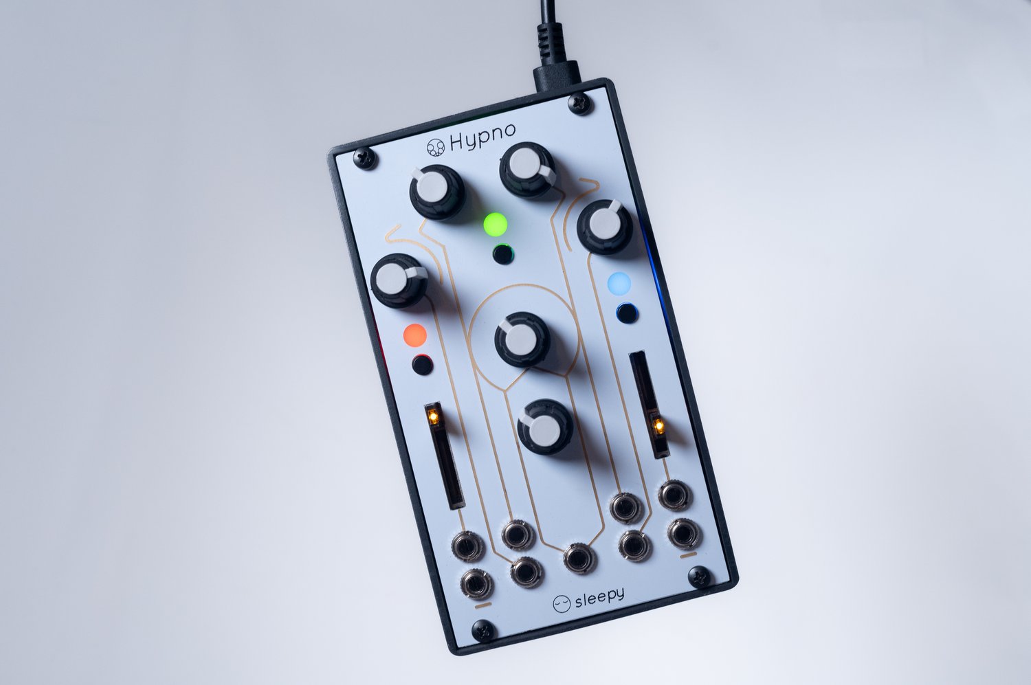
As previously stated, the face of the Hypno features two sliders, three buttons, and six dials. For convenience, through this manual, I will refer to the two sliders as A & B (left to right) and the three buttons as A, B, & C (left to right). For the dials I will refer to the four at the top as A, B, C, & D (left to right) and the two in the center as E & F (middle to bottom). The Hypno has several modes of operation that are accessed by holding down (or not holding down) buttons. I will refer to the mode where no buttons are being held down as performance mode.
image from Sleepy Circuits.
To get started with the Hypno, let’s not use any input, and just use it to generate video using its two video oscillators. The module is symmetrical, so the controls on the left (slider A, button A, and dials A & B) generally control the first oscillator, while the controls on the right (slider B, button C, and dials C & D) control the second oscillator. The controls in the middle (button B and dials E & F) generally control the module as a whole.
Buttons A & C set the shape for the two oscillators. Pressing the buttons cycles through the shapes, sine, tan, poly, circle / oval, fractal noise, and video input. These shapes are coded with the color of corresponding LED (red, green, yellow, blue, pink, and teal). The last setting, teal / video input, is only accessible when a USB video input is plugged in. We’ll deal with the video input shape in a later tutorial. While the manufacturer refers to the first two shapes as sine and tan, they both are essentially lines. The polygon shape is a septagon by default.
Red
Sine
Green
Tan
Yellow
Polygon
Blue
Circle / Oval
Pink
Fractal Noise
Teal
Video Input
A silent video demonstration of the five basic shapes in Hypno.
Sliders A & B set what the manufacturer calls frequency, but perhaps it is better understood as a zoom function. The zoom feature can be very useful when you are first getting used to the Hypno. Zooming in completely, that is pulling the slider all the way to the bottom can make a video layer disappear, so you can better see the effect of each control. Dials A & D rotate the selected shapes, and dials B & C control the polarization of the shapes. When polarization is low, the shapes appear normal. As polarization increases, the shapes start to bend until they completely wrap around, forming concentric circles. However, it should be noted that for the polygon, circle / oval, and video input shapes, dials B & C function as Y (vertical) offsets.
A silent video demonstration of the zoom, rotate and polarization / y offset controls on the five basic shapes.
The remaining two dials (E & F) control both oscillators. The former controls the gain of each shape, with the center position resulting in a black out of both layers. The latter dial controls affects the colors of the two layers, shifting the relationship between the hues of the two layers. At this point you should understand the basic shapes and controls in performance mode for the Hypno. Notice however, with the controls we have introduced thus far, there is no movement on its own. That is the shapes only change when a control (button, slider, or dial) is changed.
Here is the Sleepy Circuits quick guide for performance mode (they call it shape pages) . . .
I gave a presentation at Synthfest on November 9th, 2024 in Burlington, Massachusetts. This workshop is related to my ongoing research in using Pure Data as a tool for computer-assisted composition, sound processing, and sound synthesis. Specifically, the presentation is on how to use Pure Data to create polymetric beats. A hackable template is available below for download. You can hear such beats in my most recent album, Rotate (Bandcamp, Spotify, Apple, Amazon).
Pure Data is often used as a tool for sound synthesis or signal processing. A quick history lesson reminds us however that it is also a robust tool for algorithmic, or computer-assisted composition. Pure Data is an open source visual programming environment for sound and multimedia. It is strongly based upon the programming environment Max. When Max first added the ability to process and generate audio and video, it was referred to as Max/MSP/Jitter to highlight these new abilities. However, going back to the very beginnings of Max, originally developed at IRCAM in 1985 by Miller Puckette (who also developed Pure Data), it was centered on interactive, algorithmic and computer-assisted composition.
Defining the Problem
In order to create polymetric beats in Pure Data, it is useful to think of two steps in the process. The first is how do we represent musical patterns in a way that is easy to codify for computers. The second is how do we read that pattern in such a way that we can fire off a MIDI note at the correct time to realize that pattern.
Attached to this blog post is a program shell that we will use to understand a basic process where patterns are defined and initialized, a time structure, a structure for evaluating whether a note should happen, an algorithm for firing off a note, and a structure for changing musical patterns. The way this program shell is designed, it currently only generates kick drum parts in common time. However, once we learn how this algorithm works, we can hack it to create far more complicated beats.
Defining a Pattern
Generating rhythmic content using an algorithm is a very useful exercise, as we do not have to worry about pitch material. On the most basic level, we could think of a measure of as being a list of sixteenth notes (or whatever the fastest pulse of the desired rhythm is), and we can express the rhythm by using zeros where notes do not happen, and ones where notes are played. Thus, if we want to define a four on the floor kick drum part in common time, we could express it as . . .
1 0 0 0 1 0 0 0 1 0 0 0 1 0 0 0
When we define tables in Pure Data, the first number indicates where in the table we’re putting the values. Typically, we would want to start at the beginning of the table, which would be position 0. Thus, from now on in, I will start every rhythm description with a 0, resulting in . . .
0 1 0 0 0 1 0 0 0 1 0 0 0 1 0 0 0
This is pretty basic. If we wanted to go a bit more advanced, we could imagine two different options, a normal kick drum, which we’ll represent with the number 1, and an accented kick drum, which we’ll represent with the number 2. If we want to accent beat one of the measure, we now get the table description . . .
0 2 0 0 0 1 0 0 0 1 0 0 0 1 0 0 0
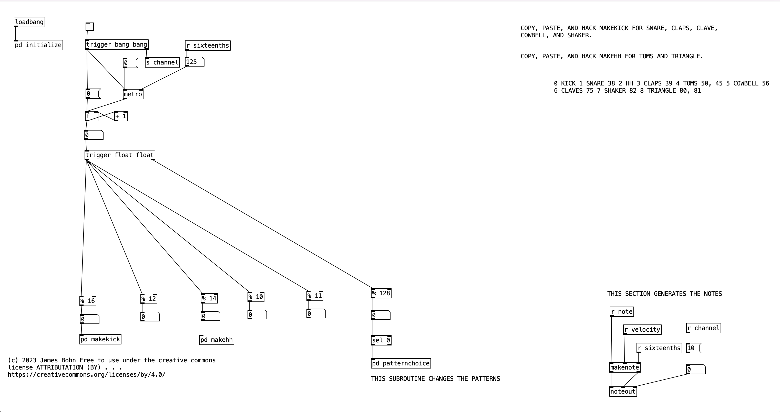
Notice, it would be pretty easy at this point to use the number zero for when notes do not occur, but use the MIDI velocity number(1-127) to indicate when a note should occur. Doing this, you can get very finely tuned dynamic drum parts. However, such subtlety is not for me, I’m more of a boom / bap / boom-boom / bap guy myself, so I will be sticking with accented and unaccented notes. Let’s look at this table definition as it occurs in the program shell. To get there, double click on the object labeled pd initialize, which is below loadbang . . .
For those who are relatively new to Pure Data, loadbang designates algorithms that execute when you open the program. Likewise, any object in Pure Data that starts with the letters pd are subroutines. Double clicking them allows you to view and edit the algorithm contained inside the subroutine. Subroutines are a great way to declutter your screen, and to create algorithms that you may want to copy and paste into other programs you create. Note that the subroutine pd initializealso sets the tempo, translates that into milliseconds, and then into sixteenth notes (still expressed in milliseconds). Finally, we also see that pd initialize contains a definition for a table called phrase, but we’ll get to that later.
Changing Patterns
Before we get to how to use this kick drum pattern, I want to introduce one more level of complexity. In the long term it would be useful to define several different kick drum patterns so we can change patterns every eight measures or so to have a dynamic drum part. As we start to add more layers to the drum part (snare, high hat, toms, etc.) it would also be nice if some of those layers occasionally did not play at all, so the combination of layers also change as we move from phrase to phrase.
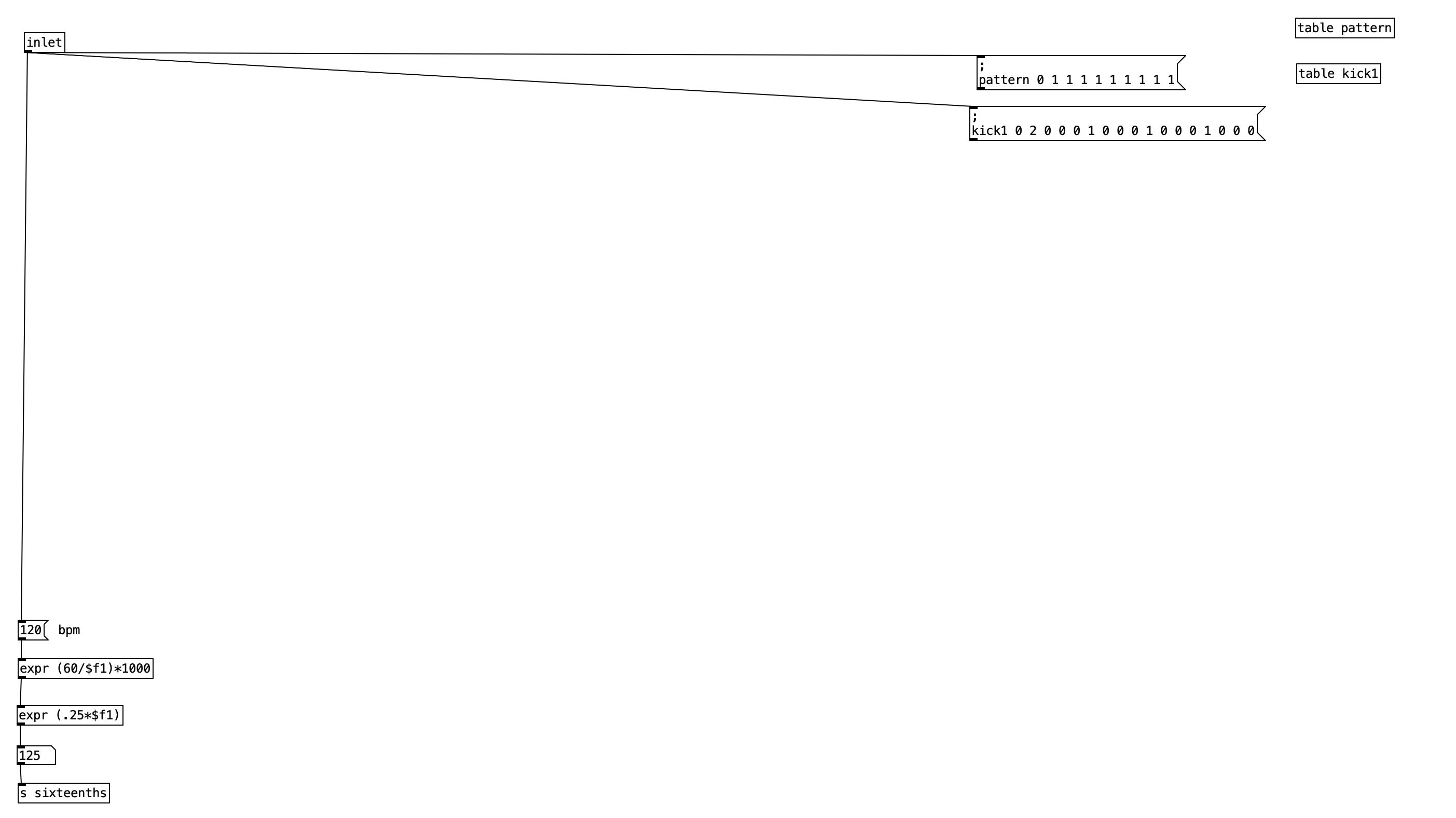
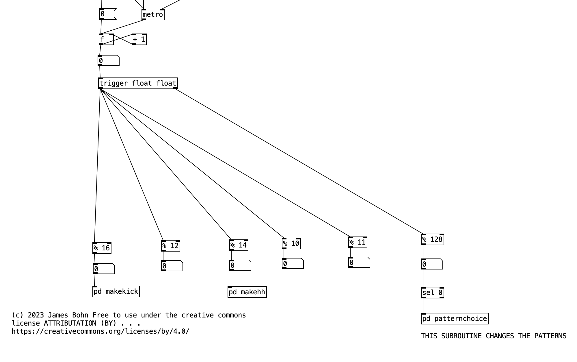
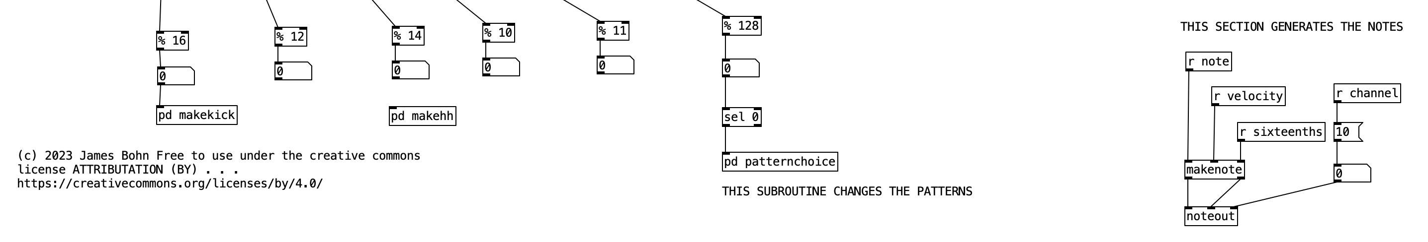
For the purposes of this algorithm, I’m going to allow for each layer of the drum part to select between three patterns (1, 2, & 3). Furthermore, I’ll also include a fourth possibility of 0, which would correspond to no pattern playing. In order to see how this is implemented in our algorithm, let’s look at the counter mechanism beneath the main metronome object. Beneath this metronome we see a trigger object, and beneath that, we see an object that states % 128. This is modular mathematics, which limits the value to a number between 0 and 127 (inclusive). We then feed the outcome of this to an object that states sel 0. When this object receives a 0 in its leftmost inlet, it will send a bang to its leftmost outlet. We then send this bang to trigger the subroutine pd patternchoice. Musically, what this means, is that the subroutine pd patternchoice executes at the beginning of every eight measure phrase. Since we are thinking in terms of sixteenth notes (8 x 16 = 128), a 0 would indicate the beginning of a phrase.
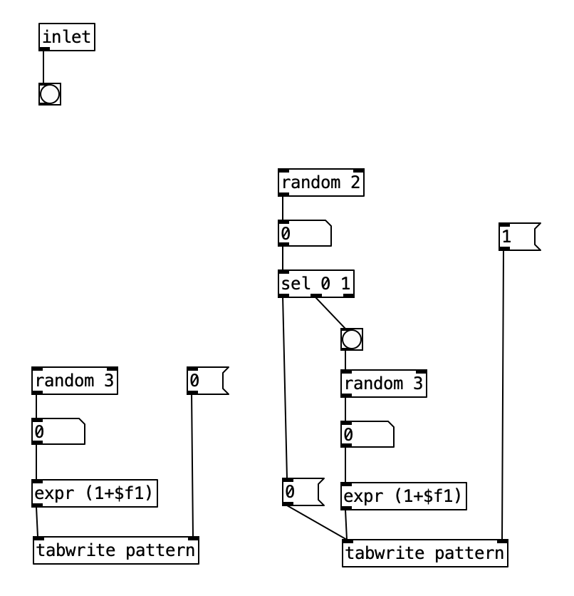
If we look inside pd patternchoice, we see two structures that are currently not connected to the inlet. In time we will copy and paste these structures, changing some of the numeric values, and connect them to the inlet. We will make these changes as we add more layers and patterns to our drum beat. However, for the time being since we only have one kick drum pattern, neither structure is connected to the inlet.
We will treat the algorithm on the left as being connected to the kick drum, while the algorithm on the right will eventually be used for the snare drum. Notice there is a difference between the two structures. The one on the left is simpler, and if we follow what it does, we figure out that that algorithm will write a 1, 2, or 3, but not a 0 to the table pattern in position 0. The structure on the right however, will write a 0 to the table patttern at position 1 half of the time. To put this into musical terms, the difference between the two means that kick drum will always be playing a pattern, while the snare drum will only play a pattern 50% of the time.
Firing Off a Note
Now lets see how pattern and kick1 are used to either fire off notes or not. We see at the bottom of the screen a makenote object connected to a noteout object that performs the final task of sending a midi note out. However pd makekick is the subroutine that determines whether or not a kick drum should occur at a given point. Above pd makekick we see the object % 16 which comes from the counter. This object mods the current counter to a number between 0 and 15 inclusive. These values correspond to the number of sixteenth notes in a measure of common time. Thus, when we return to the number 0 after the number 15 occurs it corresponds to returning to the beginning of the measure.
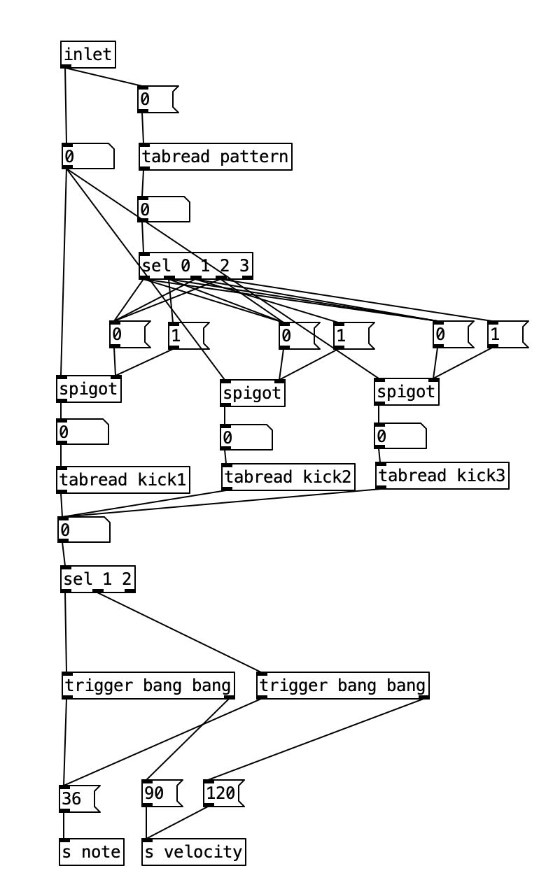
When we look at the structure pd makekick a lot of the heavy lifting of the subroutine is handled by the object spigot. Spigot receives numeric values through its leftmost inlet. However, it only passes those values through to its outlet if the numeric value being fed to its right most inlet is not zero. Thus, we can think of spigot as a valve that shuts off the flow of numbers when the rightmost inlet is zero. We can use this to selectively shut down the rest of the algorithm, which will effectively stop it from making notes.
The first step is to determine whether a pattern should be playing or not. Likewise, at the same time we can determine which patterns should be playing if one occurs. To do this, we’ll read the value of pattern at array position 0 (which we’ll use to store the current kick drum pattern). We can then route the output of that to a number of different outcomes using a sel statement. Each outcome of the sel statement sends either a 0 or a 1 to the rightmost inlet of three spigots. These spigots correspond to the three possible kick drum patterns. Thus, when the pattern is 0, a 0 is sent to all three spigots, effectively shutting off the rest of the subroutine. When the pattern is 1, we send a 1 to the spigot for pattern one (turning it on), and a zero to the other two, making sure any previously used pattern is turned off, and so fourth.
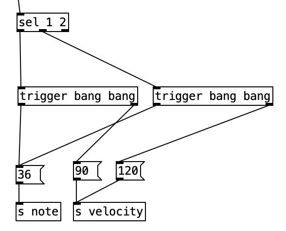
Once we pass through one of the spigots, we encounter the part of the subroutine that determines whether a note should be fired at any given time. Underneath each spigot is a tabread object that reads the current position of a given pattern (kick1, kick2, or kick3, respectively). This will return the result of a 0, 1, or 2, corresponding to no note, normal note, and accented note. Since we don’t have to do anything when no note is played, we can simply ignore that result. All we have to do is correctly route the results for 1 and 2. Since all three patterns will be outputing 0, 1, and 2, we will treat those three results the same, we can route the output of each tabread statement to the same number box, and then route the results using sel 1 2. Both results will sending the number 36 to s note (36 is the MIDI note number corresponding to a kick drum), and will send a velocity of either 90 or 120 to s velocity.
Understanding Execution Order
In order to understand the mechanics of this, we have to understand a little about execution order for Pure Data. When an outlet branches off in several directions, Pure Data first executes the connection that was created first, regardless of where it is placed on the screen (in Max, it executes from right to left). When an algorithm branches off in this way, it travels all the way down until it hits the end, and then Pure Data goes back and executes the other branch of the algorithm. When an object has multiple outlets, it typically executes the rightmost outlet first (following it all the way down the algorithm) before it most to the next outlet.
Alternately, when an object has several inlets, the object typically does not spring into action until the leftmost inlet is triggered. We can think of new values that are connected to inlets that are note the leftmost inlet as queueing until the leftmost inlet is triggered. This order of execution in Pure Data allows non-crossed connections to fire in the correct order. To illustrate, imagine an object with two outlets and an object below with two inlets (similar to the makenote / noteout algorithm below). Furthermore, let’s imagine that the right outlet is connected to the right inlet of the object below, and the left outlet is connected to the left inlet of the object below. First, the value from the right outlet will queue at the right inlet of the object below, then the left outlet will send its value to the left inlet, triggering the object below.
However, whenever we start to make complicated algorithms, it can be confusing to see in what order the algorithm will flow. When we want to force a specific order to achieve a specific outcome, or simply to make order clear, we can use a trigger object. A trigger takes a single inlet, and uses it to trigger several outlets (including the option of passing the inlet to one or more outlets) in a specific order. That order is (you guessed it, right to left). We will use this to control the order of sending the velocity and sending the note number.
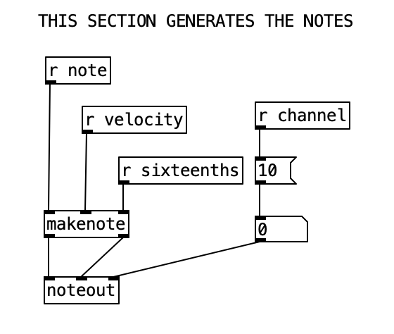
The makenote object has three inlets that correspond to midi note number, velocity, and duration expressed in milliseconds. Since midi note number is the leftmost inlet, we have to send that value last. This means we have to send the velocity before we send the note number. Here we do not have to worry about duration, since duration is often irrelevant when triggering drum samples. Thus, we can set a duration of a sixteenth note during the initialization process.
Hacking the Shell
With the knowledge we have gained thus far, we are now equipped to start hacking the program shell. A good place to start would be to double click [pd initialize], copy both the object [table kick1] and the corresponding message that populates that table. You can then paste these objects, move them so they don’t overlap, change both to say kick2 instead of kick1, and change the numbers in the in the kick2 message to be a different pattern. Again, your pattern should only use the numbers 0, 1, and 2. Likewise, the table should be 17 numbers long with the first number being 0, in order to denote that we’ll load the array starting at the beginning. You can then connect the kick2 message to the [inlet] object.
Now do the same process again creating a table and message for kick3, making sure to connect the kick3 message to inlet. Now, we can finally make use of the subroutine [pd patternchoice] in the main algorithm. Double click on [pd patternchoice], and connect the outlet of the bang to both the [random 3] object and the message that contains the number 0. Now, when we run the the algorithm, we should hear the kick drum pattern randomly change once every eight measures.
Now we can get into the good stuff. Let’s add a snare drum part. First, we should decide what meter we want to use for the snare drum. For the purposes of this demonstration, let’s put the snare drum in three. We’ll start by copying the object [pd makekick] and pasting it. More the copied object under the [% 12] object, and connect the outlet of [% 12] to the inlet of the copied object. Let’s also rename the copied object to [pd makesnare].
We have to change some details of [pd makesnare] to get it to make a snare part. Double click the object and change the message box near the top from 0 to 1. Change the array names in the three [tabread] objects to be snare1, snare2, and snare3. Finally, right above the object [s note], change the number in the message box from 36 to 38 (the MIDI note number for snare drum).
Now, double click the object [initialize], and copy the three kick drum tables, as well as the three messages that define those tables. Paste those items, and move them so they don’t overlap with other items. change the array names to snare1, snare2, and snare3 in both the table objects and the messages that define the arrays. Now, let’s change the patterns. Since these are patterns that are in three, they will feature 12 sixteenth notes. Thus, each message will have to include 13 numbers, the first being the number 0 to indicate that the pattern is loaded at the beginning of the array. Again, use 0 to indicate no note, 1 to indicate a note, and 2 to represent an accented note. Make sure you connect each of the three messages to the inlet.
Now we need to allow the snare patterns to change, so let’s double click the subroutine [pd patternchoice]. In this subroutine we need to connect the outlet of the bang to both the [random 2] object and the message that contains the number 1. The[random 2] here yields a 50% chance that the snare appear in a given phrase. The [random 3] below that will select one of the three snare patterns when it is determined that the snare should appear in a phrase.
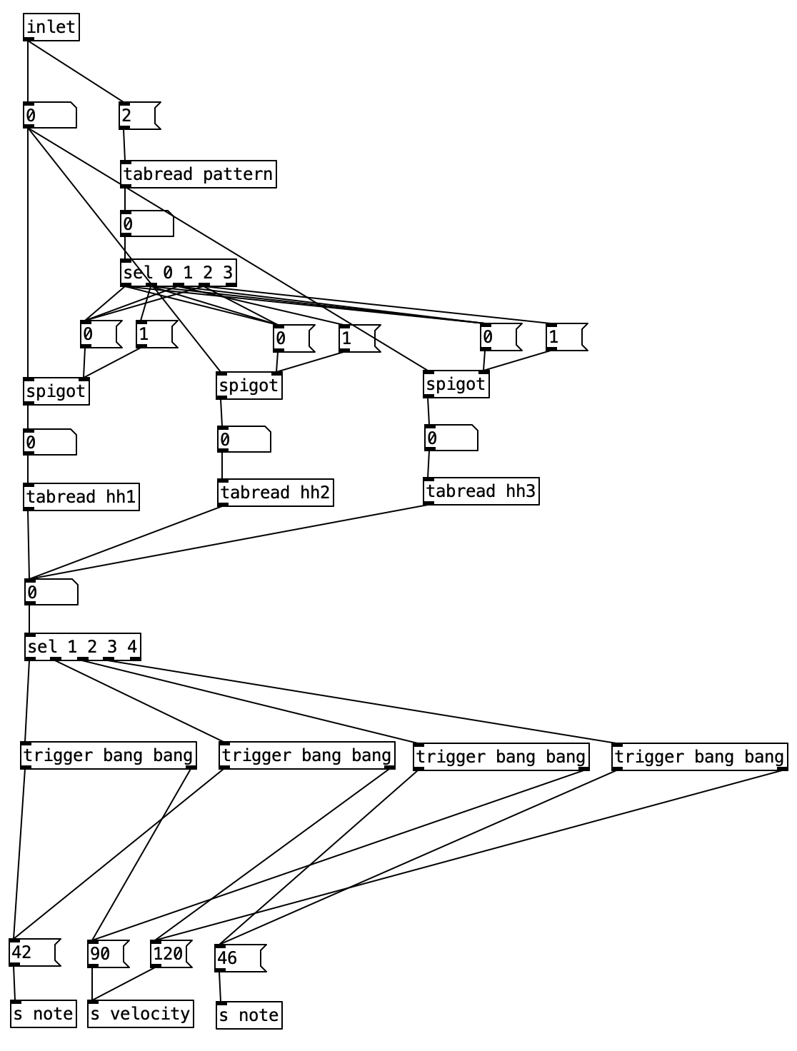
If we wanted to make a percussion part that used two different MIDI notes, we should look at the subroutine, [pd makehh]. Two notes are required for a high hat part to allow for closed and open high hats. If we look inside pd makehh, we see that the patterns allow for five possibilities, 0, 1, 2, 3, & 4. When we look at the sel statement near the bottom of the screen, the number 0 does not appear in it. Again, this is because 0 means do not play a note, so we can simply ignore that result. The way this is setup, 1 and 2 are closed high hats with the latter being accented, while 3 and 4 are open high hats with 4 being accented.
If we wanted to fully implement this subroutine, we’d have to attach it to one of the meter generators, % 16, % 12, % 14, % 10, or % 11. Then we would have to create three patterns (hh1, hh2, hh3) in [pd initialize], remembering to make the table, and use a message to populate it. You would populate the patterns using only the numbers 0, 1, 2, 3, and 4. Then you’d have to copy the block of code inside of pd patternchoice that we used to choose the pattern for the snare drum, paste it, change the index in the message object to 2, and connect the random object and the index message to the inlet.
We could also adapt [pd makehh] for creating a subroutine that will generate a toms or conga part consisting of a high tom / conga and a low tom / conga. You would have to remember to use a new / different index number to store the pattern, and change the MIDI note numbers to those corresponding to either the a high tom or conga and a low tom or conga. Ultimately we can continue in this vein, creating increasingly complicated drum beats, using [pd makekick] as a means creating layers of single note percussion parts, and [pd makehh] as a model for creating percussion layers using two different notes. As the number of meters used increases, you’ll find the resulting beats get increasingly funky, and take longer times to evolve in compelling ways, enabling you to inject rhythmic interest into your music.
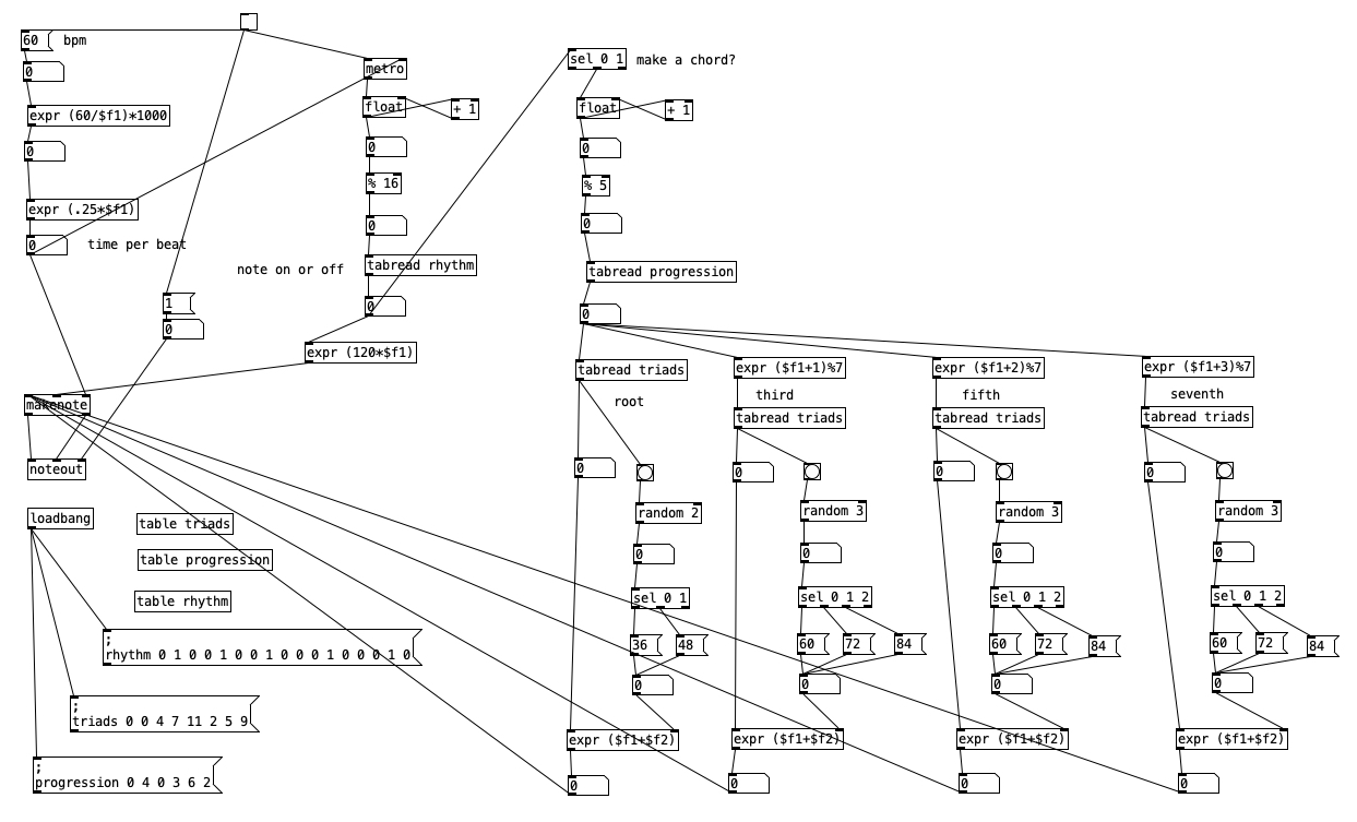
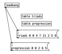
In the previous post we looked at a random arpeggiator that uses diatonic chord progressions. In this entry we will be using the same technique for creating diatonic chord progressions, but we will be applying it to create block seventh chords that repeat in a sequencer like fashion. Again we use the same code used in the scale sequencer to translate tempo from beats per minute to time per beat (expressed in milliseconds). As mentioned, we use the same table, ; triads 0 0 4 7 11 2 5 9, from the previous post to denote the notes of C Major, arranged as stacked thirds.
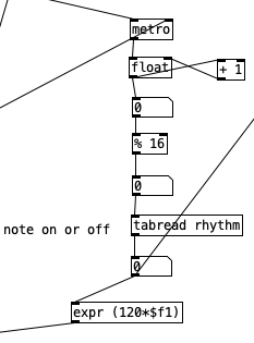
As we did in the previous patch, we can make a list of index numbers that relate to the triads table, which can be used to define the roots of a chord progression. In this case we are using the table ; progression 0 4 0 3 6 2. This results in the progression Dm7, CMaj7, Bm7(b5), Am7, G7. The other new element of this patch involves introducing a rhythmic pattern. This is accomplished using the table rhythm, where we use 1 to indicate a chord happening, and 0 to mean a rest happening. The table includes 16 numbers, indicating a single measure of sixteenth notes. The resulting rhythm starts out using syncopation where the first three chord jabs occur once every three sixteenth notes (or a dotted eighth note). The final two chords occur on the off beats of beats three and four, yielding a pleasantly funky rhythm.
We use the rhythm table table in a very simple manner. We mod the counter to 16, resulting in a sixteenth note rhythm that repeats every measure. We then read the rhythm table. Multiplying that number, which will be a zero or a one, by 120 gives us a velocity. A velocity of zero results in makenote not generating a note, while the chord stabs will be reasonably loud at 120.
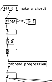
The number from tabread rhythm is then also passed to a sel statement. Remember that this note will only be a zero or a one. Thus, by using sel 0 1, and only using the outlet for 1, we only pass to the rest of the algorithm when a chord is supposed to occur. We then have a counter that is for the current chord, modding that to 5 gives us an index for reading the progression table.
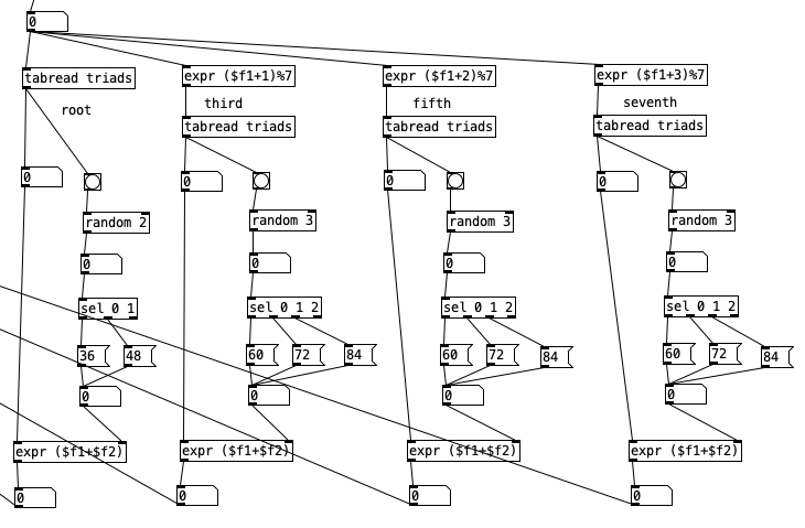
The output of tabread progression then in turn feeds four similar parallel algorithms that generate the specific notes of the given chord. These four algorithms are laid out left to right, and correspond to the root, third, fifth, and seventh of the given chord. In case of the root, the output of tabread progression and uses it as the input to tabread triads, which will yield the root of the triad. This is also added to one of two random octaves, 36 or 48 which will yield a note in the bass clef.
The other three notes add a number to the output of tabread progression. These numbers, one, two, and three, correspond to the third, fifth, and seventh of the chord. Modding that number by seven wraps any number that goes beyond the length of the table back to the beginning. The output of those expr statements then feeds tabread triads, yielding specific pitches. These pitches are added to one of three random octaves, 60, 72, or 84 to get random voicings. All four outputs of the expr statements, which give the transposed MIDI note numbers of the root, third, fifth, and seventh are fed to makenote which creates the chord when it is fed a velocity of 120. The output of this patch sounds like this . . .
In the previous post, we had an introduction to patches in Pure Data using a patch that plays a scale in quarter, eighth, and sixteenth notes in three different octaves. In this post we’ll be looking a way to generate diatonic triads using a chord progression. Again, these patches are intended to teach concepts of music theory along with concepts of music technology.
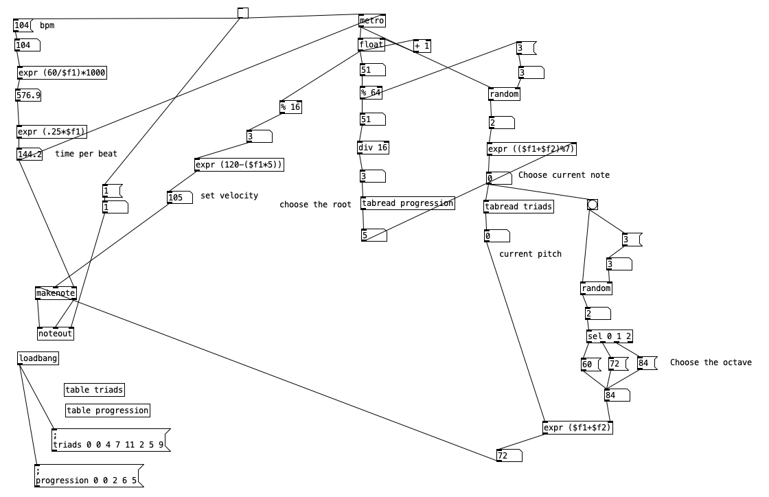
Some portions of this patch are similar to portions of the previous patch, so we’ll give them only a brief mention. For instance, the portion (in the upper left) that translates tempo (in this case 104 beats per minute) into time per beat (expressed in milliseconds) is essentially the same. Here is multiplied by .25 to yield a constant sixteenth note rhythm. Likewise, the portion of the patch that actually makes the notes and outputs them to MIDI (middle left) is essentially the same.
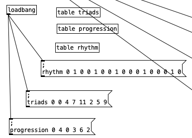
We have previously introduced loadbang and tables. Here we use tables to define diatonic triads in C Major. Using C as zero, triads 0 0 4 7 11 2 5 9 presents the notes of C major in stacked thirds (C, E, G, B, D, F, A respectively). If we pull out three consecutive numbers from this table, we will get a root, third, and fifth of a triad. We can wrap the table around to the beginning using modular mathematics (in this case mod seven) to yield thirds and fifths of the A chord, as well as the fifth of the F chord.
We can define a diatonic chord progression by noting the table position of the root of the chord in the triads table. Accordingly progression 0 0 2 6 5 gives us the roots C, G, A, and F. Given the layout of Major and minor thirds within a Major scale, this gives us the specific harmonies, C Major, G Major, A minor, and F Major. Fans of popular music will recognize this progression from numerous songs, including “Don’t Stop Believing,” “Can You Feel the Love Tonight,” and “Country Roads.”
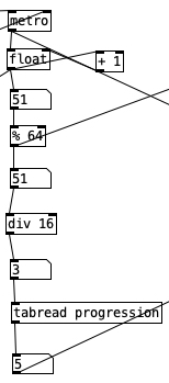
The metronome used in the patch ticks off sixteenth note increments, so the % 64 object beneath the counter reduces the counter to a four measure sequence (four groups of 16 sixteenth notes adds up to 64 notes). This number is used in the object div 16, which yields the whole number portion (non-fractional portion) of the number being divided by 16. This will result in the values 0, 1, 2, or 3. This is essentially the current measure number in terms of the direction. Feeding this to tabread progression. Will give the index value for the root of that measure’s chord when used with the triads table.
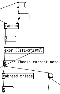
The value from the tabread progression object is sent to the right inlet of the expr statement in the segment above. A random number between 0 and 2 inclusive is fed to the left inlet of the same expr statement. The random number represents whether the note created will be a root (0), a third (1), or a fifth (2). by adding these two values together we get the index of the specific pitch the triads table. Using mod 7, % 7 in the expr statement, insures that if we go beyond the end of the the triads table that we will wrap around the beginning of the table. This index is then passed to tabread triads, which returns the numeric value of the specified note.
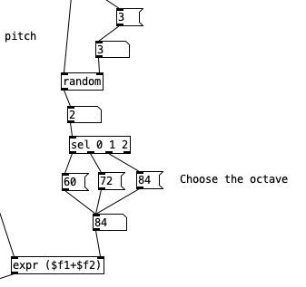
Note that in the previous segment a second outlet from the number object beneath the expr statement is then sent to a bang. This activates the random code in the segment above, namely the selection of a random number between 0 and 2 inclusive. This number is passed to a sel statement, specifically, sel 0 1 2. This object activates one of the three leftmost outlets, depending upon whether it is passed a 0, 1, or 2 (respectively left to right). the rightmost outlet activates if anything besides 0, 1, or 2 is encountered. In this case we pass the three left most outlets to three messages, 60, 72, and 84. These numbers are three different octaves of C (middle C, C5, and C6 respectively). Those messages are fed to a number object, which in turn is fed to the right inlet of an expr statement. The left inlet of this expr statement comes from the output of tabread triads. Thus, in expr ($f1+$f2) the pitch is added to one of three octaves, yielding a random arpeggiation across three octaves of pitch space. Let’s listen to the results of this patch below.