During the month of February I rewrote the third phrase of the pedal steel part for Landscape 2: Snow. I unfortunately did not have any time to record any new tracks for the project. I do plan on recording a bass part over spring break. I do have some updated audio to share this month. Appropriately enough it is Landscape 2: Snow. This realization includes a guitar part performed by Carl Bugbee of the prominent Rhode Island cover band Take it to the Bridge, and the cello part is played by Dr. Nara Shahbazyan who performs in the Providence based New Music group Ensemble Parallax.
Landscapes Update: February 1st, 2020
During January I revised Landscape 1: Forest by adding a musique concrete layer. The sound sources I used include horn recordings from Landscape 7: Mountains, as well as bass harmonica recordings from Landscape 4: Sand Dunes. In all cases, I used Audacity to change the pitch level, as well as to stretch out the samples. My plans for February include revising the pedal steel part for Landscape 2: Snow. I’ll leave you with an updated realization of Landscape 1: Forest, including the new musique concrete layer.
Feedback in FM Synthesis
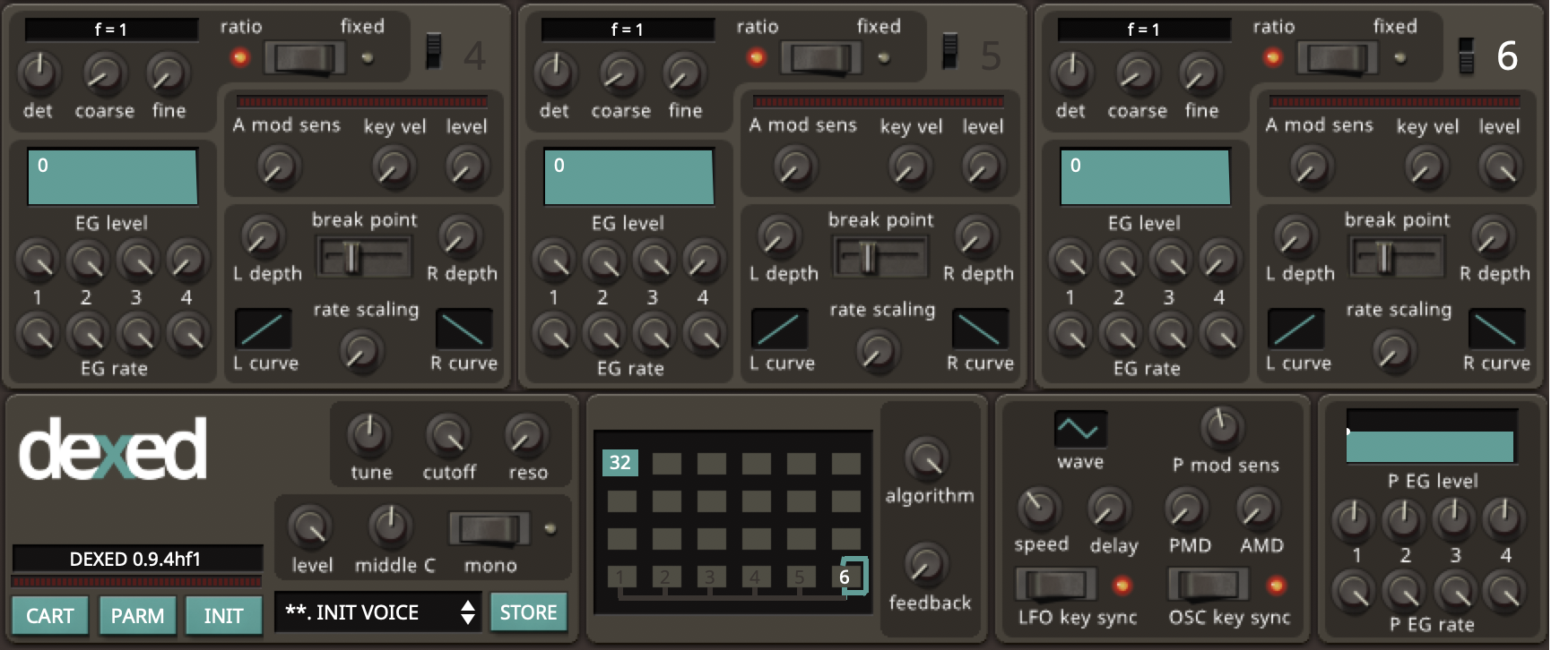
FM Synthesis can be difficult to understand. Those of us who spent time programming a Yamaha DX7, the leading FM synthesizer of the 1980s, also know how confusing it can be to program. Fortunately for those who are nostalgic for classic synthesizers of the 1980s Digital Suburban develed Dexed, a DX7 emulator.
The good news is that Dexed works just like a DX7, allowing you to port over classic patches. The bad news is that Dexed works just like a DX7, in that it can still be confusing and awkward to program. However, the better you understand FM synthesis, the better equipped you’ll be to tackle Dexed.
In this post we’ll investigate feedback, which in FM synthesis is when some of the output an operator is fed back to modulate itself. In a DX7, there are eight levels of feedback available (0-7 inclusive). No feedback is present at level 0, while at level 7 there is (presumably) 100% feedback.
I tested feedback in Dexed by using algorithm 32, which is the only algorithm in which a carrier modulates itself. I turned off all the operators except for operator six, which is set at full volume, and at a ratio of 1.00 (the first harmonic). Each pitch is at A4 (440Hz) with full velocity.
It is interesting to see and hear the results of the test. Predictably at feedback level 0 a simple sine wave results. At feedback level 1 the second harmonic starts to appear at less than 1/4 the strength of the first harmonic. At feedback level 2, this second harmonic somewhat stronger (at approximately 1/4 strength). At feedback level 3, the first four harmonics are present with the strength of each being about 1/3 the strength of the previous harmonic. At feedback level 4, the harmonic spectrum of the first eight partials of a sawtooth wave become recognizable. We get the first 18 partials at level 5. At level 6 we get what could be called a hyper sawtooth wave, with a very strong peak at partial 34, with lesser peaks running up from partials 26 through 46. Finally, at level 7 we get a white noise spectrum with added strong partials at the first two harmonics.
This analysis bears out when looking at the resulting waveforms in Audacity. We start with a pure sine tone, and with each increase of the level we start to see the sine wave lean to the left a bit. By feedback level 3, a smoothed sawtooth wave is clearly visible. At level 5 we see a pretty close approximation of a sawtooth wave. The waveform at level 6 appears to be 34 periods of sawtooth waves shaped into sawtooth wave type shape at the frequency of the first harmonic. Furthermore, we get a significant amount of positive side DC offset in the waveform, leading to some distortion (we had actually gotten some DC offset at level 5 as well). The waveform at level 7 has a clear profile of white noise, though it seems to have occasional fragments of a noisey square wave. Interesting enough we also get a small amount of negative side DC offset.
Ultimately, what we learn is that feedback shapes an oscillator’s sine wave into a sawtooth wave, peaking at level 5, moving into a hyper sawtooth wave at level 6, and becoming largely white noise at level 7.
Landscapes Update: January 1st, 2020
So I finished the composing for the Landscapes project on December 14th, 2019. Or did I? My wife, who teaches writing, would tell anyone that the key to good writing is revision. Any part that has already been recorded I will consider to be finished, but I plan on making at least one revision every month to one of the Landscapes movements. One of the things I may add is a layer of Musique Concréte to some movements, as it may make the pieces more marketable to festivals and conferences, and it’ll add another layer of timbral interest.
I plan on writing a grant for 2021 that will fund recording efforts for the Landscapes project. Until then I intend on continuing to record parts for the movements on my own. Accordingly, in December I finished a recording of the bass part for Landscape 5: Marsh, which is included below. Today I have made a YouTube playlist of the Landscapes project, so if you wish to hear them continuously, you may. I will continue to post updates on the Landscapes project every month or so, and will update the playlist as I add more recordings. Anyway, as promised, here is a recording of Landscape 5: Marsh featuring Carl Bugbee (from the prominent Rhode Island cover band Take it to the Bridge) on electric guitar, and myself on electric bass.
Low Pass Filter Demonstration
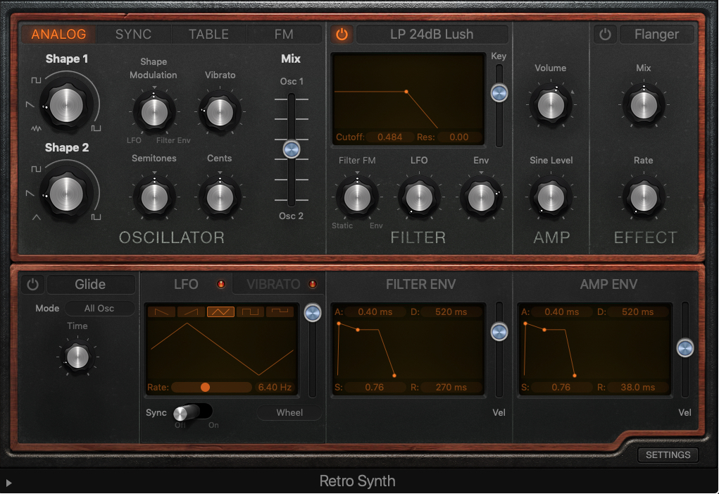
Of the various filters used in subtractive synthesis, the low pass filter is by far the most commonly used. Accordingly it is useful to examine how this filter alters sound. To that end, I’ve made a couple of videos that demonstrate three different filters in Logic Pro’s Retro Synth instrument.
Before getting too deep in the process, I’ll start with some basic information. A low pass filter attenuates frequencies above a set center frequency. Filters are often described in terms of their slope, that is the amount that higher frequencies are attenuated. Slope can be described in terms of decibels per octave. Thus, a 24dB filter dampens frequency content by 24 decibels per octave. To put it another way if the center frequency is set at 100 Hz, audio at 200 Hz should be attenuated by 24 decibels, while audio at 400 Hz should be attenuated by 48 decibels. Thus, the higher the slope, the more effective the filter is at attenuating filtered frequency content. Slope can also be described in terms of poles, which translates out to 6dB. Accordingly, a 24dB filter is also called a 4 pole filter, while a 12dB filter is called a 2 pole filter.
The three filters demonstrated in these videos are a 24dB low pass (described as being Lush), a 12 dB low pass (described as being Creamy for some unknown reason), and a 6dB low pass (described as being Lush). Each is demonstrated with a 4 second, 55 Hz sawtooth wave (A1, where C4 is middle C). In each pass, the center frequency is swept up from the lowest to the highest frequency setting for the filter. Thus, we hear harmonics add in over the course of four seconds.
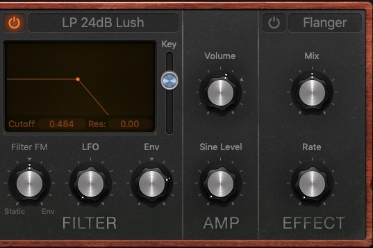
Additionally, these videos also demonstrate how the filters in question respond to difference resonance settings, which begs the question, what on God’s green earth is resonance? Resonance feeds the audio at the center frequency of the filter back through the filter. At moderate settings this can allow harmonics to be accentuated when the center frequency matches the frequency of a sound’s harmonic. At very high settings quality analog filters self resonate, which means they produce a sine wave at the center frequency even when no sound is patched into the filter. Because resonance creates a peak at the center frequency, it can increase the perceived slope of a filter. Each video features nine passes, three for each filter (24dB, 12dB, and 6dB respectively). The first pass of each group features no resonance, while the second has the resonance set at 50%, and the final has the resonance set at 100%.
What do we learn from these videos? While it would be technically incorrect to say that these filters all self resonate, we can say that they are coded to emulate self resonating filters, so for all intents and purposes, these filters are functionally self resonating. Thus, when the resonance is turned up to 100% we hear a sine tone sweep up the entire frequency range of the filter in addition to the filtered 55Hz sawtooth wave. Furthermore, we can see that sweep in a linear fashion in Logic’s graphic equalizer, confirming it responds in a linear fashion in pitch space, or exponentially in frequency space. The resulting wave form is basically a sine wave laid out over the structural form of a longer period sawtooth waveform. One odd thing we notice is that the 12dB (Creamy) filter peaks severely when the resonance is turned up to 100%. I found this to be true at every key velocity.
We also hear that the filters effectively accentuate harmonics when the resonance is set at 50%. This allows us to hear the exponential curve of the filter. As the center frequency moves up linearly in terms of octave pitch space, it accentuates increasing numbers of harmonics as the more harmonics are grouped within an octave as you sweep up the frequency range.
We can also hear and see how much more effective the higher slope filters are than the lower slope filters. We can see how the higher slope filters effectively squelch higher frequencies when the center frequency is low. Likewise, we can see how much more curved the output waveform is when the center frequency is low.
Here we can see the waveforms as each filter is tested . . .
Here we see the spectral analysis of each tone as evolves in Logic Pro . . .
So Much Noise
Did you know that there is a technical definition of noise? Did you know that there are six main colors of noise? The most common type of noise is white noise, which consists of random fluctuations such that there is equal energy content per bandwidth. This can be thought of as being similar to a flat frequency response. Pink noise consists of random fluctuations with equal energy per octave. Brown (also called Red) noise consists for random fluctuations where the energy level of each bandwidth is related to the squared inverse of the frequency (1/f2). When listening to these three types of noise, it sounds like pink and brown noise are progressively lower in frequency than white noise. That is because more of their energy is concentrated in lower frequencies in comparison to white noise.
Blue noise features energy levels that are proportional to frequency, resulting in a 3dB increase per octave. Violet (or Purple) noise utilizes energy levels that are proportional to the square of the frequency, resulting in a 6dB increase per octave. When comparing blue and violet noise to white noise, they will sound higher in frequency than white noise, as increasing amounts of their energy is concentrated in higher frequencies. Finally, Grey noise is basically white noise that has been filtered to correspond with equal loudness curves, so that the while the energy level of each bandwidth will not be measurably equal, but will be perceived by human beings as being the same loudness.
To demonstrate white noise, I generated four seconds in Logic Pro’s Retro Synth. You can listen to the results below. On the first pass, the waveform is displayed in Audacity, on the second pass it is displayed as a spectrum in Logic Pro.
Landscapes Update: December 1st, 2019
Landscape 12: Autumn Forest is complete, and I have started the first phrase of Landscape 13: River, which will be the last piece in the series. I edited and mixed an orchestral reading of Landscape 7: Mountains. The reading, which was done in early November, was by the Musiversal Lisbon Orchestra https://www.musiversal.com/).
There’s been some changes on the Musiversal front. They are discontinuing the 30 piece Lisbon orchestra, and are adding a different 30 piece orchestra. This comes with some good news and some bad news. The bad news, as a consumer, is that they are raising their prices a bit. However, this is really good news, when you worked out how little the musicians were getting paid, they really do deserve more money. On the good side of things, they are allowing composers to purchase only seven minutes of time again, rather than having a 14 minute minimum, making it a bit more economical.
They’re also changing the instrumentation a bit. The new 30 piece orchestra only has 2 horns instead of 4, but they are adding a harp and percussionist. I’m actually pretty enthusiastic about that change. I don’t get to write for harp much, and who doesn’t love some timpani? Accordingly, I recomposed the orchestral part I wrote for Landscape 10: Rocky Coast, which I will hopefully have read in late winter 2020.
I’ll leave you with the new realization of Landscapes 7: Mountains with the added orchestral part, as well as Carl Bugbee’s guitar tracks. This piece was a bit tricky. Four phrases in work have orchestral backing. Two of these feature a dotted quarter hemiola, so I rewrote these to be in a compound meter in a different tempo to avoid syncopation in the orchestral part. Another difficulty for the piece is that it is in Gb major. However, only one of the phrases was easily notated in concert Gb major. Given instrumental transposition, it made the most sense to notate the other three phrases in E major, and add sharps where needed. Ultimately it made the most sense to write each phrase with a measure of rest of the entire orchestra between phrases, and to put the phrases in a different order than they appear in the piece in the arrangement. Even though two of the phrases segue into each other, it was easier to have the orchestra record them in separate passes, and edit them together in LogicPro.
Oscillator Sync in Subtractive Synthesis
Did you ever wonder what oscillator sync does in subtractive synthesis? Simply put, in sync mode oscillator 2 restarts its waveform every time oscillator restarts its waveform. That’s pretty simple to understand, but it is a bit trickier to visualize, and harder still to try to predict what the auditory outcome will be.
Thus, I have done a test of oscillator sync using Logic Pro’s RetroSynth. Each test involves two passes, each of which is 16 seconds long. Both instances use 55 Hz sawtooth waves (A1, where middle C is C4). In the first pass, we are listening only to the synced oscillator. In the second pass, we hear a 50/50 mix of oscillator one and two.
In both cases however, I am automating the sync value. For all intents and purposes, each pass starts out with the frequency of the synced oscillator matching that of oscillator one, and gradually increasing until at the end of the 16 second pass, the frequency of oscillator two is about sixteen times the frequency of oscillator one.
Watching the audio while it plays in Audacity (below), we see on the first pass, long period sawtooth waves gradually shorten into shorter period sawtooth waves. This change will be audible in an apparent rise in frequency. On the second pass, you’ll see these increasingly shorter period sawtooth waves superimposed on the long period sawtooth wave of the first oscillator.
As we watch a spectral analysis of the sound displayed in an EQ plugin on the output channel of Logic Pro (below), we will see each successive harmonic of the 55 Hz fundamental rise in volume as the first pass progresses. You’ll notice that the rate of those harmonic peaks increases over the course of the pass. This illustrates that the sync knob of RetroSynth is exponential in nature, that is it moves up the frequency spectrum using consistent octaves, not consistent frequency bands. For instance in first octave of motion (55 Hz through 110 Hz), we have two harmonics represented (55 Hz & 110Hz). In the second octave of motion (110 Hz- 220 Hz), we have three harmonics represented (110 Hz, 165 Hz, and 220 Hz). In the next octave (220 Hz through 440 Hz) we have 5 harmonics presented (220 Hz, 275 Hz 330 Hz, 385 Hz, and 440 Hz), and so forth. Thus, more harmonics are presented in the same span of time, giving the aural impression of speeding up. You should hear these harmonics cycle though the harmonic series. On the second pass, you’ll see the same thing, only with the fundamental 55 Hz tone constantly there, softening the feeling of the frequency increasing a bit.
Ultimately, the increased angularity of the sound waves, as seen in Audacity results in a richer harmonic content (as seen in the harmonic analysis). This demonstrates the point of Oscillator sync in subtractive synthesis, namely to create richer harmonic content than what is available in the basic waveforms of subtractive synthesis.
Subtractive Synthesis Waveforms in Logic Pro’s RetroSynth
If you’re like me, you may wonder, how accurate are the waveforms in LogicPro’s RetroSynth subtractive synthesis emulator. It turns out, they’re pretty accurate. I tested the sine, triangle, sawtooth, square and pulse waves. At first glance, RetroSynth seems to only offer triangle, sawtooth, square, and pulse waves (noise as well, but that’s for another day) . . .
However, if you look at the amplifier portion of the emulator, there is a knob labeled “Sine Level.” Thus to get a sine wave, you have to pull down the filter CF all the way to the bottom, and pull up the Sine Level . . .
For the test I put in a whole note with a key velocity of 100 for each waveform. I used the note A1 (middle C=C4), resulting in a 55 Hz tone. You can see and hear the results in this video . . .
Note however that there are some weird artifacts during the square wave, which come from data compression.
Those of you who know your waveforms know that a sine tone is a pure tone that has no overtones (harmonics). A triangle wave is a sum of all the odd harmonics, where the fundamental is harmonic 1, with the amplitude of each partial is 1/(n squared). A sawtooth wave features all harmonics with an amplitude of 1/n. A square wave includes all the odd numbered harmonics with the amplitude of 1/n. A pulse wave is a variable square wave, and the harmonic content is reliant upon the width of the pulse. I used a graphic equalizer in Logic Pro to display the harmonic content of each waveform.
Landscapes Update: November 3rd, 2019
Hello all! I have finished my writing quota for October, so Landscape 11: Farmland is complete. I’ve started working on November’s goal, Landscape 12: Autumn Forest, completing the first phrase. I have also written an orchestral part for Landscape 10: Rocky Coast, which will likely get recorded in Spring 2020.
Last month I finished spending the budget for my grant, with Carl Bugbee recording the guitar part to Landscape 8: Palm Glade, and Nara Shahbazyan recording cello parts for Landscapes 2 and 6 (Snow and Beach) respectively. Next weekend the orchestral part for Landscape 7: Mountains will get recorded by Musiversal’s Lisbon Orchestra. Thus, there will be some great musical updates that I’ll share with you all in the future, but for this month, I’ll share with you Landscape 8: Palm Glade featuring Carl Bugbee’s guitar tracks!